Understanding cultural persistence and change: a replication of Giuliano and Nunn (2021)

Giuliano and Nunn (2021) provide econometric evidence that ancestral climatic variability reduces the current importance of tradition. We conduct a “deep reproduction”, comparing the precise descriptions of the individual-level regressions in their article with the corresponding code. This analysis uncovers several major inconsistencies, also related to the code not included in their replication package. A published corrigendum addresses some inconsistencies we had also communicated to the Editor of REStud, but several remain, relating to a substantial portion of the observations. A realignment of the code with the text reveals a more nuanced relationship between ancestral climatic variability and tradition.
Cultural persistence, Tradition, Deep reproduction
Acknoweldgements
The replicated article is: Paola Giuliano and Nathan Nunn (2021), “Understanding cultural persistence and change,” The Review of Economic Studies, 88(4), 1541-1581. The code underlying this replication is available at: https://www.openicpsr.org/openicpsr/project/202861. We are grateful to Paola Giuliano and Nathan Nunn for their engagement in our replication exercise and for providing valuable feedback to us. The content of our exchanges remains private, as we did not ask for their consent to share it. We also appreciate the comments provided by the Guest Editor, Abel Brodeur, and by two anonymous referees, as well as those received from Toman Barsbai, Denis Cogneau, Yannick Dupraz, Jesús Fernández-Huertas Moraga, Francesca Marchetta, and Jérôme Valette. We acknowledge the support received from the Agence Nationale de la Recherche of the French government through the program Investissements d’avenir* (ANR-10-LABX-14-01). The usual disclaimers apply.
1 Introduction
Cultural persistence, the preservation of cultural traits over time, is a topic of profound importance in economics and social sciences. Research has demonstrated the enduring influence of culture on economic outcomes, such as female labor-force participation and fertility decisions. Moreover, harmful practices rooted in tradition may hinder social progress.
The study published in The Review of Economic Studies by Giuliano and Nunn (2021) (henceforth GN, the Authors, or the original article) has garnered significant attention in economics due to its novel insights into the determinants of cultural persistence. Drawing inspiration from evolutionary anthropology, GN propose that societies that have historically experienced greater climatic variability exhibit lower persistence of cultural traits. This prediction stems from the idea that intergenerational environmental changes reduce the value of knowledge embedded in tradition, rendering it less relevant to current conditions.
To test this hypothesis, GN employs a combination of theoretical modeling and econometric analyses using multiple data sources. The core of their empirical approach focuses on natives of immigrant origin residing in the United States, who provide a unique opportunity to study the effects of historical climatic variability on cultural persistence.1 By comparing immigrants from different countries with varying climatic histories but living in the same location, GN can isolate the impact of climatic variability from other confounding factors related to geography. Additionally, the analysis incorporates data on Native Americans to address concerns about unobserved heterogeneity across different countries due to different patterns of self-selection into migration to the United States from different origin countries.
The findings of GN consistently support the evolutionary anthropology prediction. They show that greater ancestral intergenerational climatic variability experienced by one’s ancestors is associated with lower levels of cultural persistence, as measured by various indicators of the importance of tradition and the adherence to cultural norms. Empirically, all the results presented in GN point to a consistent negative effect of the ancestral intergenerational climatic variability experienced by one’s own ancestors on various stated and revealed measures of the importance of tradition as well as on the persistence of cultural norms. These results highlight the crucial role of past environmental factors in shaping the persistence of cultural traits.
GN’s theoretical model and empirical findings have become keystones in economics, inspiring multiple articles to explore the implications of their insights. The original article has already been cited extensively, despite its recent publication, with Google Scholar reporting 364 citations and publisher metrics showing that it has received approximately 64 times more citations than the average publication in the same field (information retrieved on March 14, 2024). These citations include influential articles published in leading journals, for instance, Bau (2021), Bazzi et al. (2019), Bazzi et al. (2020), Bazzi et al. (2023), Bursztyn et al. (2024), Caprettini and Voth (2022), Enke (2019), Ghosh et al. (2023), Michalopoulos and Xue (2021) and Valencia Caicedo (2018).2
Paralleling its bibliometric impact, its scientific contribution is substantial. Indeed, economists are increasingly coming to understand the long-term impact of ancestral cultural traits on contemporary outcomes. In that respect, this literature provides numerous empirical pieces of evidence of the persistence of culture across generations. On the other hand, another vivid literature presents numerous examples of rapid cultural change, such as the Protestant Reformation (see the introduction in GN), or the abandonment of traditional values following the contact with Europeans, or the implementation of national policies (Bau 2021). GN represents a pioneering effort to answer the central and natural question that arises: when does culture persist, and when does it change?
In this article, we present the results of our “deep reproduction” (Dreber and Johannesson 2023)3 of some of the econometric results reported by GN. As defined by Dreber and Johannesson (2023), “deep reproducibility studies, [dig] deeply into the original study including the raw data and the coding decisions to detect potential coding errors or questionable coding decisions.”4
This type of reproduction is desirable because, as Krähmer et al. (2023, 2) points out, “[o]pen code alleviates two problems that currently compromise the credibility of research: Errors in data preparation and misspecifications of statistical models. While model misspecification should, in principle, be discernible from the body of an article, errors in data preparation are downright impossible to spot without access to authors’ code.” This approach aligns with Clemens’s (2017) definition of replication, where researchers use the “same” specification, population and sample as in the original article.5 Indeed, within this framework, we conduct a replication test which “include: fixing coding errors so that the code does exactly what the original paper describes (verification)” (Clemens 2017, 329). Moreover, as Huntington‐Klein et al. (2021) argue, researcher degrees of freedom, such as decisions made during data collection, preparation, and analysis, can lead to variation in results, even when replicating the same study. Accordingly, we thoroughly verified the correspondence between the specifications described in the original article and the code and estimation sample provided in the replication package of GN. Importantly, this verification was not limited to the analysis code but also extended to the data cleaning and manipulation procedures, which were not included in the replication package. By closely examining the documentation and the data, we were able to reverse-engineer certain aspects of the data processing, even in the absence of access to the original code. For example, we identified instances where variables that should have been constant over time or across subgroups of observations exhibited variations, thus revealing that the actual data manipulation is inconsistent with the description provided by GN.
The replication exercise relies on three main elements: the original article by Giuliano and Nunn (2021), a corrigendum published in The Review of Economic Studies (Giuliano and Nunn 2024), and the replication package of the original article, which can be accessed at https://doi.org/10.5281/zenodo.4026093. The latter includes the estimation samples used to estimate each equation, together with the corresponding codes.6 However, it does not include the raw data, the code necessary to transition from the raw data to the various estimation samples, and the codes that generate the results reported in the online Appendix of GN.
The corrigendum was published after our exchanges with the Authors and with the editor in charge of the original article. The Authors write “[s]ince the publication of the article, imprecisions in wording and omissions in the text have been pointed out.” (p. 597).7 However, as will become apparent in the following discussion, the corrigendum: (i) deals with only a minor subset of the inconsistencies that we had signaled to the Authors and to the Editor in charge of the original article, (ii) does not describe the implications of these imprecisions for the econometric exercises conducted in the original article, and, in some instances, (iii) generates inconsistencies with other portions of the text of the original article that have not been modified. Throughout the following discussion, references to page numbers, equations, and tables correspond to the original article unless otherwise specified. Similarly, references to line numbers pertain to the file GiulianoNunn_replication.do included in the replication package.
1.1 Our reproduction approach
The characteristics of the replication package have shaped the scope of our replication exercise. Specifically, our focus lies on two key aspects: (i) the results reported in the main text and (ii) the estimation of all the six equations using individual-level data. Point (i) arises from the absence of the code to reproduce the online Appendix within the replication package, limiting our analysis to the results presented in the main text alone. Point (ii) stems from the absence of data cleaning and manipulation codes in the replication package, making it considerably more challenging to identify potential inconsistencies between the article’s text and the excluded code that pertains to aggregate data.8 Moreover, according to the Authors, regressions comparing “individuals with different cultural backgrounds but who live in the same city in the U.S.”(Giuliano and Nunn 2021, 1543) are superior.9 For these reasons, (iii) our focus lies on the discrepancies between code and text (i.e., a deep reproducibility) rather than the replication of the estimates because the codes and data provided on the original replication package do not allow to fully do the latter.
Our replication provides detailed citations from the original article to document the precise and unambiguous descriptions of the specifications used in the six equations estimated with individual-level data. We then identify any inconsistencies between these textual descriptions and the actual code or estimation sample used.
We identified two main types of inconsistencies between the code and text. The first type concerns errors in the analysis code included in the replication package, such as deviations from the specified estimation sample or variables that were impossible to construct according to the original article. The second type relates to problems with the data cleaning and manipulation code, including issues with the estimation sample, variables with distributions at odds with the text, and missing or incorrectly constructed variables. These inconsistencies are discussed in more detail in the subsequent sections.
We have identified and documented inconsistencies within the six equations we analyzed, which correspond to four distinct tables and a total of 28 data columns.10 Discrepancies greatly vary in terms of their empirical relevance (see Figure 1–Figure 3).
The remedies we propose to address the uncovered discrepancies are straightforward: doing so simply needs to adhere to the precise and unambiguous descriptions provided in the original article. However, it is not feasible to solve all the issues due to the lack of essential variables in the replication package.11 As a result, we are unable to fully re-estimate the equations in a manner consistent with the original article. Nonetheless, we want to emphasize that the exercise we present is a “deep reproduction” of the original article, and documenting these errors indicates that the original article cannot be replicated, regardless of any possible changes in the estimated coefficients.12
It is important to clarify that we do not take a position on whether the specification described in the original article or the one actually implemented in the code is more economically sound. Our thorough reproduction aims to compare the text of the original article, which has undergone peer review, with the corresponding code. The scope of our analysis is limited to this comparison, and it does not evaluate the merits of the possible alternative specifications. Furthermore, we would like to highlight that the published corrigendum (Giuliano and Nunn 2024) has also been validated by The Review of Economic Studies, and we refer to its content below. Lastly, we want to clarify that, we never propose or run any specifications that deviate from those described in the paper.
The rest of the paper contains six short sections, each corresponding to one equation. These are followed by a section documenting the impact of the corrections on the estimates in GN, and by a concluding section.
2 The six equations using individual-level data
For each equation, we first identify and describe the coding discrepancies. We then compute the share of observations affected by each discrepancy in the estimation sample used in each data column,13 and propose a method to realign the code with the original article’s specifications. In our online Appendix, we document the incidence of each discrepancy and present the regression results obtained by correcting all correctable errors. For each data column except for those corresponding to Equation 2,14 we provide a figure illustrating the impact of each identified discrepancy (and combinations thereof).
Eq. (2) Importance of tradition
GN write that, when estimating Equation 2 using data from the World Values Survey (WVS):
\[ \tag{1}\]
“After matching respondents’ self-reported mother tongue from the WVS with ethnicity from the Ethnographic Atlas, we estimate:
\[ Tradition_{i,e,c}=\alpha_c+\beta_2 {Climatic\ Instability}_e+ \mathbb{X}^{\prime}_i\Phi+\mathbb{X}^{\prime}_e\Omega+\epsilon_{i,e,c} \tag{2}\]
where \(i\) denotes an individual who is a member of the historical ethnic group \(e\) and lives in country \(c\). \({Tradition}_{i,e,c}\) is the self-reported importance of tradition, measured on an \(1-6\) integer scale and increasing in the importance of tradition.” (p. 1557, bold emphasis added).
Coding mistake
- (Incidence: undetermined)15 The WVS does not provide information on mother tongue. Instead, it only asks about the language that the respondent normally speaks at home.
The corrigendum reads: “On page 1557, ‘mother tongue’ should be ‘language spoken at home’” (Giuliano and Nunn 2024). We note that, for individuals of immigrant origin (i.e., foreign-born individuals and natives of foreign ancestry), the language spoken at home is a choice. Indeed, the Authors use this choice as a revealed measure of the attachment to tradition among natives of foreign ancestry in Equation 5 and Equation 6.16 Individuals of immigrant origin who are, according to the Authors, less attached to tradition are, therefore, more likely to be incorrectly assigned to the same ancestors as the natives of the country in which they reside. We refer the reader to Bertoli et al. (2024), where we propose an approach, departing from a deep reproduction, to gauge the relevance of the coding mistake that we identify for Equation 2 in GN, which cannot be directly corrected.
Eq. (4) Within-group marriage
\[ \tag{3}\]
[The] sample comprises all married women in all waves of the March Supplement of the Current Population Survey (CPS) [from 1994 to 2014] with at least one parent who was born outside the US. […] \[ {I}^{In\ group\ Marriage}_{i,c,k}=\alpha_k+\beta_3 {Climatic\ Instability}_c+\mathbb{X}_c\Pi +\mathbb{X}_{c,k}\Omega+\mathbb{X}_{i}\Phi+\epsilon_{i,c,k} \tag{4}\]
[…] The outcome of interest, \({I}^{In\ group\ Marriage}_{i,c,k}\), is an indicator variable equal to one if an individual’s spouse was born in origin country \(c\) or if his or her mother or father was born in country \(c\). \(\alpha_k\) denotes the inclusion of residence (i.e. metropolitan-area) fixed effects. The vector of country-level covariates \(\mathbb{X}_{c}\) includes the natural log of the current per-capita GDP in the country of origin (measured in the survey year) […] [\(\mathbb{X}_{c,k}\)] includes the fraction of the population in the same metropolitan area as the individual who are first- or second-generation immigrants from the same country of origin.” (p. 1562, bold emphasis added).
Coding mistakes
(Dependent variable, incidence between 2.0 and 2.8 percent) The dependent variable in Equation 4 is created in a portion of the code not included in the replication package. Its definition requires information on the country of birth of the spouse and of the parents-in-law. The March Supplement of the CPS provides this information exclusively for individuals co-residing with their spouses,17 but the estimation samples in Table 4 include married individuals not co-residing with the spouse, with the dependent variable for them being either equal to 0 or to 1. It is not possible to create the dependent variable in a way consistent with its description provided at p. 1562 for married individuals whose spouse is absent.
(Fraction of the population, incidence of 100 percent) The control variable measuring “the fraction of the population in the same metropolitan area as the individual who are first or second-generation immigrants from the same country of origin” (p. 1562) has actually been computed separately for each year from 1994 to 2014.
(GDP 2014 - incidence between 7.9 and 8.7 percent18) The “natural log of the current per-capita GDP in the country of origin (measured in the survey year)” is entirely missing for the year 2014. Consequently, all the observations corresponding to this year are incorrectly excluded from the estimation sample.19
(Missing MSA 1, incidence between 17.0 and 19.2 percent) The estimation samples in the four data columns of Table 4 include individuals who reside in metropolitan areas that are not separately identified. These areas are represented by the
metareavalues 9997 (Other metropolitan areas, unidentified), 9998 (NIU, household not in a metropolitan area) or 9999 (Missing data). The corrigendum reads: “On page 1562, the sentence ending in ‘denotes the inclusion of residence (i.e. metropolitan-area) fixed effects’ should be followed by the clarifying footnote: ‘Rural locations within the United States do not have an MSA code. Throughout the paper, we treat a missing MSA as a category in the residence fixed effects’” (Giuliano and Nunn 2024). It also should be noted that even after the corrigendum, the statement: “[b]y examining individuals who live in the same location, we are able to hold constant the contemporaneous local environment, while examining the effects of an individual’s ancestral environment” (p. 1564) remains factually incorrect. This is because the code pools together individuals for whom the variablemetareais equal to 9997, 9998 or 9999 irrespective of their actual locations within the United States. Finally, the corrigendum does not clarify whether these three different values of the variablemetareaare treated as distinct categories in the residence fixed effects.(Missing MSA 2, incidence between 17.0 and 19.2 percent) The control variable that measures “the fraction of the population in the same metropolitan area as the individual who are first or second-generation immigrants from the same country of origin” (p. 1562) cannot be meaningfully defined for observations where the variable
metareais equal to 9997, 9998 or 9999. Additionally, this variable is not constant for individuals associated with the same foreign country \(c\), surveyed in the same year, and for whommetareais equal to (for example) 9997. This inconsistency contradicts the implication of the corrigendum that these values of the variable are treated equally to the other non-missing values.
Correcting the coding mistakes
(Dependent variable) The observations for which the variable
marstis equal to 2 (Married, spouse absent) should be excluded from the estimation sample. This correction is feasible.(Fraction of the population) The control variable should be defined in a time-invariant way. This correction is unfeasible (using the replication package).
(GDP 2014) The data cleaning and manipulation code could be easily fixed. This correction is unfeasible (using the replication package), as the replication package only mentions the data source but not the exact identifier of this variable.
(Missing MSA 1) The observations for which the variable
metareais equal to 9997, 9998 or 9999 should be excluded from the sample. This correction is feasible, but no change in the code is needed on the basis of the corrigendum.(Missing MSA 2) The control variable should be defined in a way that does not vary, when the variable
metareais equal to 9997, 9998 or 9999, across observations corresponding to a unique value of \(c\). This correction is unfeasible (using the replication package).
Eq. (5) Speaking a foreign language at home
GN estimate the following equation on a sample of individuals born in the United States and reporting a foreign ancestry in the 2000 census:
\[\begin{split} {I}^{Foreign\ Lang.}_{i,c,k}=\alpha_k+\beta {Climatic\ Instability}_c+\mathbb{X}_c\Pi +\mathbb{X}_{c,k}\Omega+\mathbb{X}_{i}\Phi+\epsilon_{i,c,k} \end{split} \tag{5}\]
“where \(i\) denotes an individual, \(c\) his/her ancestry, and \(k\) a location of residence (metropolitan areas). The dependent variable, \({I}^{Foreign\ Lang.}_{i,c,k}\), is an indicator that equals to one if a language other than English is spoken at home. \(\alpha_k\) denotes the inclusion of residence (i.e. metropolitan areas) fixed effects. [In footnote 24] We omit from the sample individuals from origin countries with English as an official language. \(\mathbb{X}_c\) denotes ancestral country-level covariates: historical distance from the equator, historical economic development, historical political complexity, the GDP in the country of origin measured at the time of the survey, and the linguistic distance between the country of origin and the U.S.” (p. 1565, bold emphasis added).
Coding mistakes
(English, incidence between 3.7 and 5.8 percent) The sample used to estimate Equation 5 includes natives with ancestry in seven distinct countries or territories (out of 84) in which English is an official language.20
The corrigendum reads:
“4. On page 1565, for the text ‘report their ancestry as being a non-English speaking country,’ the word ‘country’ should be ‘group’.
- In footnote 24, the text ‘individuals from origin countries with English as an official language.’ should be ‘individuals from ancestries with English as an official language and the language of instruction in higher education.’ ”
The corrigendum amending the original article changes the sample selection criterion, shifting it from the level of the ancestral country to the level of each ancestral group. This modification requires defining the official language and language of instruction in higher education for each ancestral group. However, the corrigendum does not specify the data source used to implement this sample selection criterion, resulting in a lack of precise description of the specification of Equation 5, unlike in the original article.
Through personal communication with the Editor in charge of the original article, it was brought to our attention that, concerning Canada, the estimation only included natives of French Canadian ancestry and disregarded individuals who defined themselves exclusively as being of Canadian ancestry.21
Moving the sample selection criterion from the level of the ancestral country to the level of the ancestral group, as Giuliano and Nunn (2024) do, also breaks the symmetry with respect to the construction of the elements in the vector \(\mathbb{X}_c\), which includes “ancestral country-level covariates”. This discrepancy is evident for
lingprox_dominant_a, a variable used inTable5.dtameasuring “the linguistic distance between the country of origin and the U.S.” is borrowed from “linguistic proximity between dominant groups (Fearon data)”. As English is the dominant language in Canada, this implies that observations for French Canadians, identified byisocode=="CAN", have a value oflingprox_dominant_aat 15 (i.e. the one associated to English), the highest value in the data.22Therefore, according to Giuliano and Nunn (2024), French Canadians are included in the sample as this group does not have English as its official language, even though the value measuring linguistic proximity is determined using English for Canada.
(Missing MSA 1, incidence between 25.0 and 32.2 percent) The estimating sample includes observations for which the variable
metareadis equal to 0 (Not identifiable or not in an MSA). A unique value of the fixed effect \(\alpha_k\) is incorrectly assigned to these observations, bundling them together. The corrigendum addresses this point, as described with respect to Equation 4 above.(Missing MSA 2, incidence between 25.0 and 32.2 percent) The vector \(\mathbb{X}_{c,k}\) includes a variable measuring the “fraction of those living in the same metropolitan area who are first-generation immigrants of the same ancestry” (p. 1565). This variable is incorrectly defined for the observations for which the variable
metareadis equal to 0.(Fraction, incidence between 25.0 and 32.2 percent) The variable measuring the “fraction of those living in the same metropolitan area who are first-generation immigrants of the same ancestry” (p. 1565) varies across individuals from the same country of ancestry, and for which the variable
metareadis equal to 0 (Not identifiable or not in an MSA).(Living with parents, incidence undetermined) Cols. (2) and (3) in Table 5 estimate Equation 5 separately for individuals not living and living with parents.23 The sample split is done, at lines 106–108, using the variable
relatedescribing the relationship of individual \(i\) to the household head. Thus, the subsample of individuals “Living with parents” includes all the individuals who are children of the household head, while the subsample “Not living with parents” includes all other individuals. For three-generation households, the split is incorrect when, for instance, a grandchild of the household head co-resides with at least one of her parents, or when the household also includes a parent of the household head. In these two cases, the grandchild and the household head are incorrectly classified by GN as “Not living with parents”.
Correcting the coding mistakes
(English) The correction can be implemented by utilizing the variable
isocodeto identify and exclude observations associated with countries and territories where English is an official language. The correction is feasible.(Missing MSA 1) The observations with a value 0 for the variable
metareadshould be excluded from the sample. This correction is feasible, but no change in the code is needed on the basis of the correction.(Missing MSA 2) The observations with a value 0 for the variable
metareadshould be excluded from the sample because the control variable cannot be meaningfully defined for these observations. The correction is feasible.(Fraction) The fraction of the population in the same metropolitan area that are first or second-generation immigrants from the same country of origin should be treated equally to the other non-missing values. In particular, it should be time-invariant. The correction is unfeasible (using the replication package).
(Living with parents) The correct sample split and the exact identification of a co-residing parent is possible using the variables
momlocandpoploc, which are available from IPUMS USA (Ruggles et al. 2023).24 This correction is unfeasible (using the replication package).
Eq. (6) Speaking a foreign language at home (living with parents)
“We estimate whether the intergenerational transmission of the tradition of speaking one’s ancestral language is affected by climatic instability of the ancestral country […]:
\[\begin{split} {I}^{Foreign\ Lang.}_{i,c,k}=\beta_1 {Climatic\ Instability}_c+\beta_2 {I}^{Parent\ Foreign\ Lang.}_{i,c,k}+\\+ \beta_3 {I}^{Parent\ Foreign\ Lang.}_{i,c,k}\times {Climatic\ Instability}_c+\\+\mathbb{X}_c\Pi +\mathbb{X}_{c,k}\Omega+\mathbb{X}_{i}\Phi+\alpha_k+\epsilon_{i,c,k} \end{split} \tag{6}\]
[…] \({I}^{Parent\ Foreign\ Lang.}_{i,c,k}\), which is an indicator variable that equals one if either the father or the mother speaks a foreign language at home.”
Coding mistakes
Equation 6 inherits the five coding mistakes described above with respect to Equation 5:
(English, incidence between 5.3 and 5.8 percent)
(Missing MSA 1, incidence between 25.0 and 26.1 percent)
(Missing MSA 2, incidence between 25.0 and 26.1 percent)
(Fraction, incidence between 25.0 and 26.1 percent)
(Living with parents, incidence undetermined)
Correcting the coding mistakes
The coding mistakes can be fixed as described with respect to Equation 5.
Eq. (8) Indigenous populations speaking a traditional language
\[ \tag{7}\]
For a subsample of individuals who report a Native American tribal affiliation drawn from the 1930, 1990 and 2000 censuses,
“[the] estimating equation is:
\[ \begin{split} {I}^{Native Lang}_{i,e,k}=\alpha_k+\beta {Climatic\ Instability}_e+\mathbb{X}_e\Pi +\mathbb{X}_{i}\Phi+\epsilon_{i,e,k} \end{split} \tag{8}\]
where \(i\) denotes an individual, \(e\) his/her ethnic group, and \(k\) a location of residence (metropolitan area). The dependent variable, \({I}^{Native Lang}_{i,e,k}\), is an indicator that equals to one if the individual reports speaking an Indigenous language at home. The specification includes location (i.e. metropolitan areas) fixed effects, \(\alpha_k\). Thus, the variation used to estimate \(\beta\) is across individuals from different Native American ethnic groups, but living in the same location. [in footnote 30] The 1930, 1990 and 2000 US Censuses ask the following question: ‘Does the person speak a language other than English at home?’ If yes, the person indicates which language.” (p. 1571, bold emphasis added).
Coding mistakes
(Language, incidence between 7.3 and 16.9 percent) The questionnaire of the 1930 census did not include the two questions necessary to define the dependent variable in Equation 8.25 For instance, the sample used in Col. (1) of Table 7 to estimate Equation 8 includes 11,468 obs. (9.0 percent) drawn from this census, and corresponding to 83 Native American ethnic groups.
Until September 2021, IPUMS USA incorrectly coded the variable
languagefor the 1930 census using the information on the mother tongue.26 In reality, the question about the mother tongue should have been asked in 1930 only to foreign-born individuals.27 However, it appears that some enumerators may not have followed this restriction.28The replication file reveals that the dependent variable is always equal to 0 for 68 of these 83 ethnic groups in 1930. Furthermore, two groups, namely Navajo and Hopi, account for the great majority (1,860 out of 1,951) of the observations where the dependent variable in Equation 8 is equal to 1 in 1930.29 This very strongly suggests that the question about mother tongue was not systematically asked to all Native Americans in the 1930 census.30
(Children 0 to 4, incidence between 3.0 and 21.4 percent) The language questions used to define \({I}^{Native Lang}_{i,e,k}\) are specifically asked to individuals aged 5 and above in the 1990 and 2000 censuses.31 However, in the estimation sample, there are observations corresponding to children aged 0 to 4 for whom \({I}^{Native Lang}_{i,e,k}\) is always equal to 0, although it should have been marked as missing since the language questions are not applicable to individuals in this age group.
(Employment, incidence between 0.1 and 61.1 percent) The question regarding employment status, which is used to define an element of the vector \(\mathbb{X}_{i}\) in Equation 8, is only asked to individuals aged 16 and above in the 1990 and in the 2000 census.32 In the estimation of Equation 8, the observations where the variable
empstatis not available are treated as a separate category of this categorical variable. This differs from what is stated on p. 1572, where the Authors mention that labor-force-status fixed effects have three values: employed, unemployed, and outside of the labor force.(Missing MSA, incidence between 60.2 and 75.3 percent) In the estimation sample, there are observations for which the variable
metareais equal to 0, indicating that the location is “Not identifiable or not in an MSA.” The corrigendum addresses this issue, as explained in relation to Eq. (4) above. We note that the statement “the variation used to estimated \(\beta\) is across individuals from different Native American ethnic groups, but living in the same location” (p. 1571) is factually incorrect, and not modified by the corrigendum.(Living with parents, incidence undetermined) “Estimates of Equation 9 are reported in columns 1–3 of Table 7 for all individuals (column 1), those not living with their parents (column 2), and those living with their parents (columns 3).” (p. 1572). The split of the sample is done on the basis of the variable
relateat lines 153 and 155 in the replication file. The remarks related to the fourth mistake for Equation 5 and Equation 6 also apply here.
Correcting the coding mistakes
(Language) The variable
yearcan be used to exclude the observations corresponding to the 1930 census. The correction is feasible.(Children 0 to 4) The variables
ageandyearcan be used to exclude observations corresponding to children aged 0 to 4 drawn from the 1990 and the 2000 censuses. The correction is feasible.(Employment) The variables
ageandyearcan be used to exclude observations corresponding to children aged 0 to 15 drawn from the 1990 and the 2000 census. The correction is feasible.(Missing MSA) The observations in which the variable
metareais equal to 0 should be excluded from the sample. This correction is feasible, but no change in the code is needed on the basis of the corrigendum.(Living with parents) The correction for the fourth coding mistakes in Equation 5 and Equation 6 should also be applied to address this issue. The correction is not feasible (using the replication package).
Eq. (9) Speaking a traditional language (living with parents)
“We again explore the transmission of this cultural practice [speaking an Indigenous language at home] from parents to children by estimating: \[ \begin{split} {I}^{Native\ Lang}_{i,e,k}=\alpha_k+\beta_1 {Climatic\ Instability}_e+\\ +\beta_2 {I}^{Parent Native Lang}_{i,e,k}+\beta_3 {I}^{Parent Native Lang}_{i,e,k} \times {Climatic\ Instability}_e+\\ +\mathbb{X}_e\Pi +\mathbb{X}_{i}\Phi+\epsilon_{i,e,k} \end{split} \tag{9}\]
where all variables are defined as in Equation 8 and \({I}^{Parent Native Lang}_{i,e,k}\) is an indicator variable that equals one if individual \(i\)’s parents speak an indigenous language at home.” (p. 1572).
Equation 9 is estimated for individuals drawn from the 1930, 1990 and 2000 censuses reporting an affiliation to a Native American tribe and “living with parents” (p. 1572).
Coding mistakes
Equation 9 inherits the five coding mistakes described above for Equation 8:
(Language, incidence between 13.8 and 16.9 percent)
(Children 0 to 4, incidence between 16.0 and 17.0 percent)
(Employment, incidence between 59.1 and 59.2 percent)
(Missing MSA, incidence between 73.0 and 75.3 percent)
(Living with parents, incidence undetermined).
Correcting the coding mistakes
The coding mistakes can be fixed as described with respect to Equation 8.
Impact of the corrections
Our “deep reproduction” exercise reveals significant discrepancies between the original study’s reported results and those obtained using the textual definitions provided in the article, even after accounting for the content of the corrigendum. We now examine the consequences of these discrepancies for the validity of the original study’s findings. In particular, we investigate how the identified issues affect the statistical precision, \(p\)-values, and magnitude of the original estimates. By doing so, we provide a comprehensive understanding of the implications of our reproduction failure, shedding light on the robustness of the original study’s conclusions.
To facilitate the exposition of the consequences of reproduction failure, we opt for a graphical representation of the results rather than the more traditional tabular format. This choice is motivated by the complexity of the errors identified, which often involve multiple corrections for each equation. Creating a table to analyze the impact of each error separately would imply generating a multitude of tables, akin to the original, but correcting one mistake at a time. Furthermore, we can also correct several errors and combinations of errors, making a tabular presentation cumbersome. Instead, we create figures that provide a concise and intuitive visualization of the results.
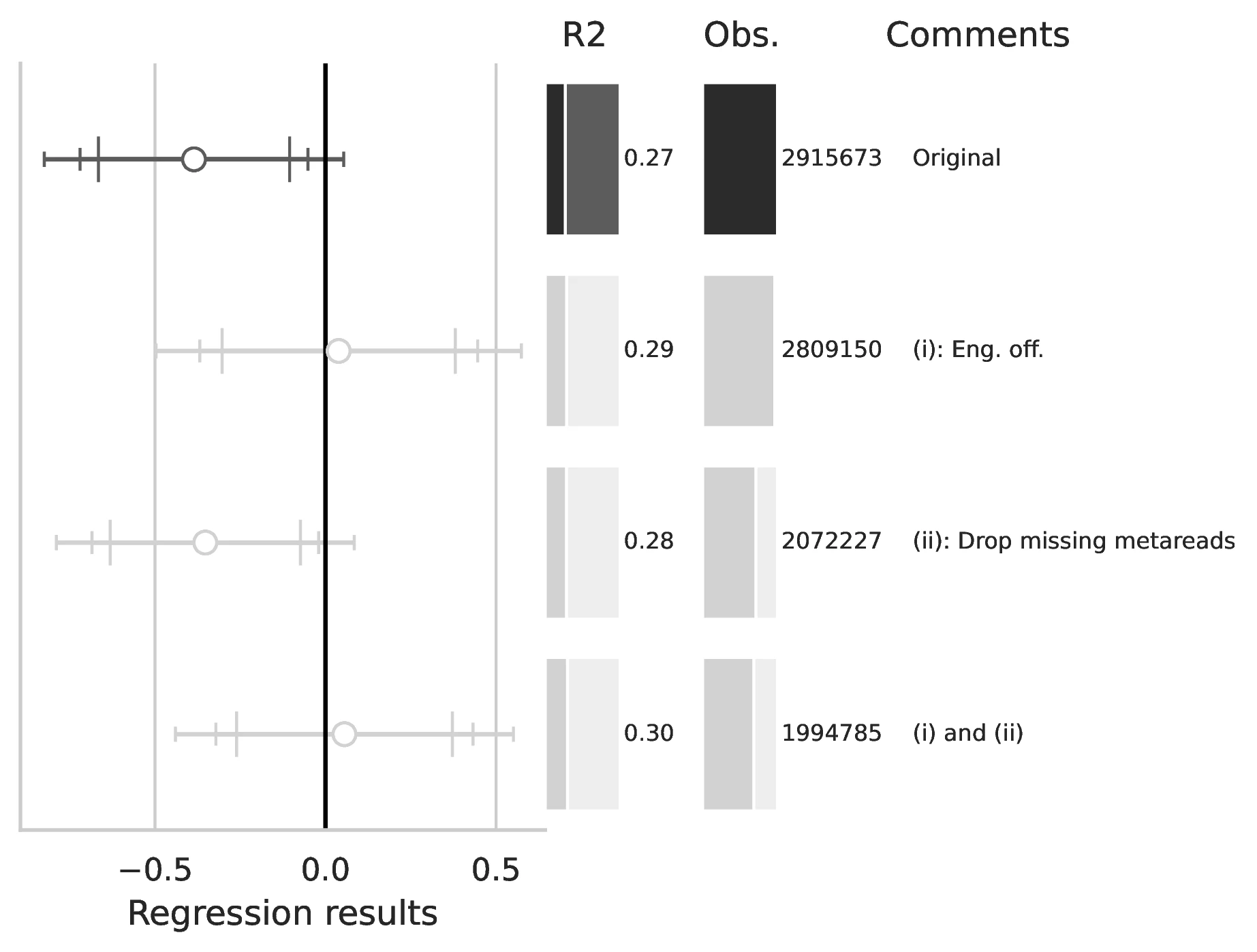
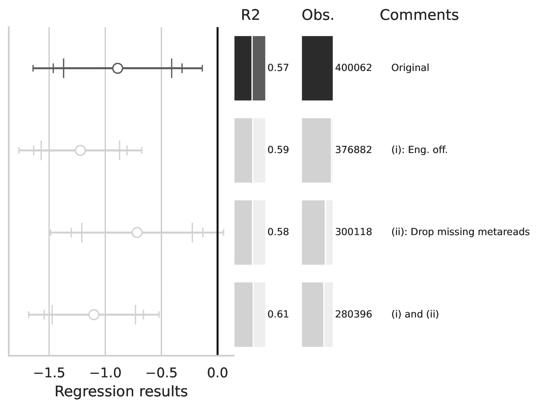
For each targeted specification, we generate a figure that compares the original estimation with the corrected results. The figure displays the original estimation, including confidence intervals, in red, alongside the corrected results, in blue. The graphical representation also includes information on sample size and \(R^2\), with a section for comments on the corrections implemented. The corrected results are presented relative to the baseline, original regression. Figure 1 provides an overview of the impact of each error in Table 4, Figure 2 focuses on Table 5 whereas Figure 3 centers on Table 7. Additionally, Table 3 and Table 4 in our Online Appendix present the results of Table 4 after implementing the (feasible) corrections we identified in previous sections.33 Similarly, Table 5 present the corrected estimates corresponding to Table 5. Finally, Table 6 and (tbl:replication_tab_7_v2?) display the coefficients of Table 7 once the corrections are introduced.34
Our “deep reproduction” exercise reveals a total of 26 coding mistakes in the original study. Notably, 53.5 percent of these mistakes (14 out of 26) could be fixed using the codes and data provided in the original replication package. Upon correcting the coding mistakes, we observe substantial changes in the estimates, with some coefficients undergoing dramatic shifts in magnitude and significance. In particular, Table 5 appears to be rather fragile to our proposed corrections, with 5 out of 7 results loosing significance once all corrections are introduced. For instance, the coefficient on the main variable of interest changes from -0.767 to -0.427 in Col. (3), a 38 percent decrease in magnitude, and becomes insignificant. The remaining tables are impacted to a lesser extent. Overall, applying the corrections, 53.0 percent of the main estimates (9 out of 17) become indistinguishable from zero, highlighting the significance of these errors for the validity of the original study’s findings.

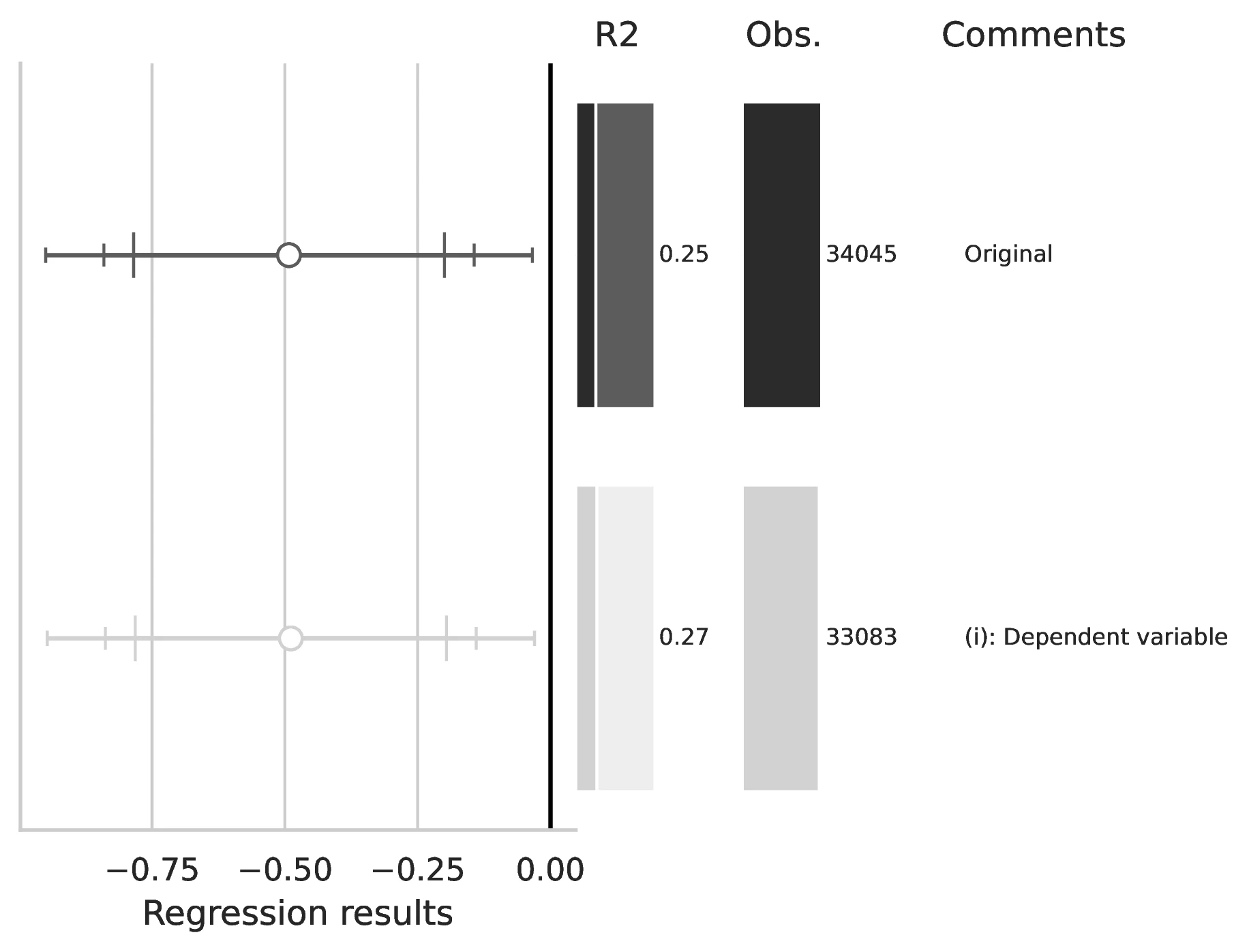
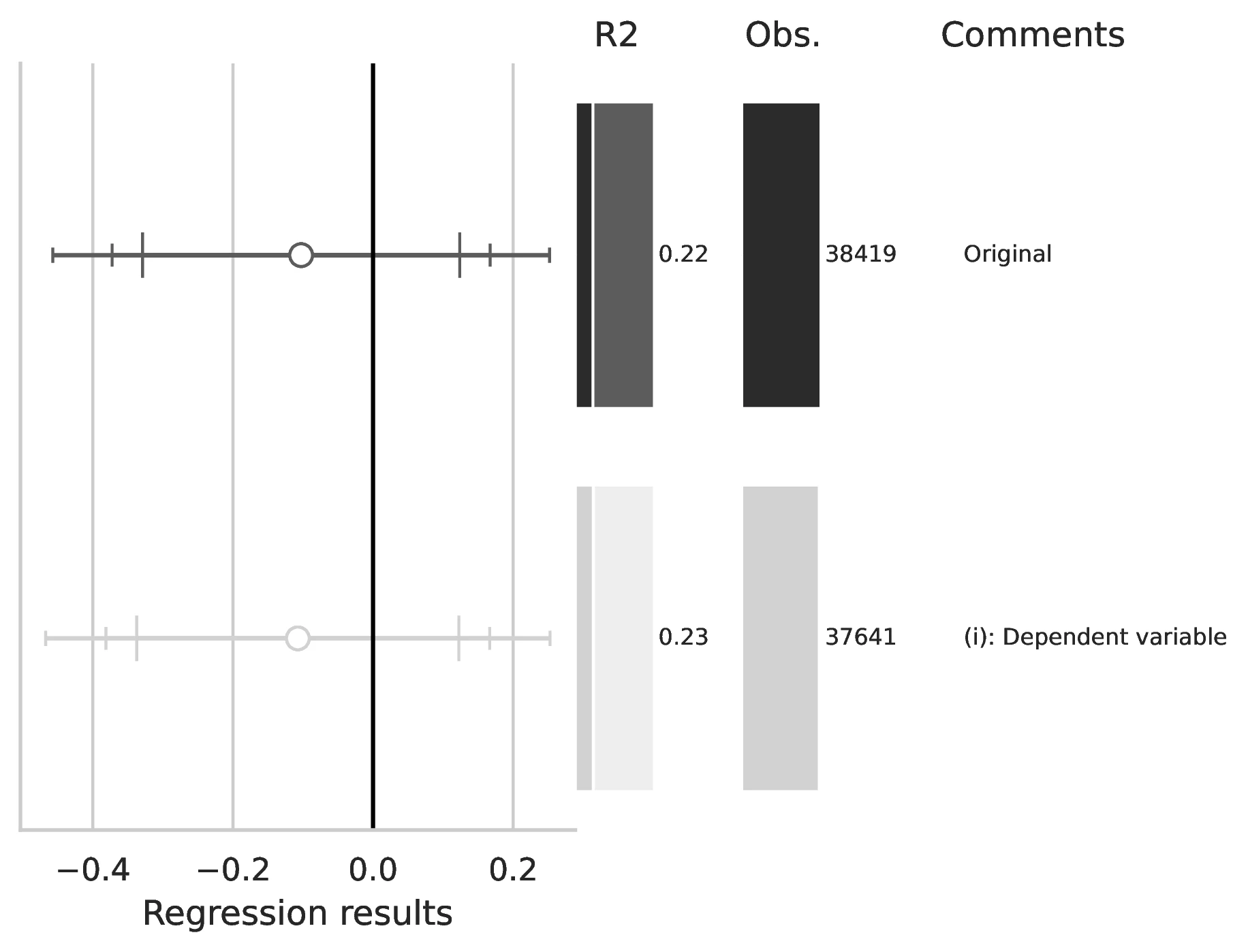
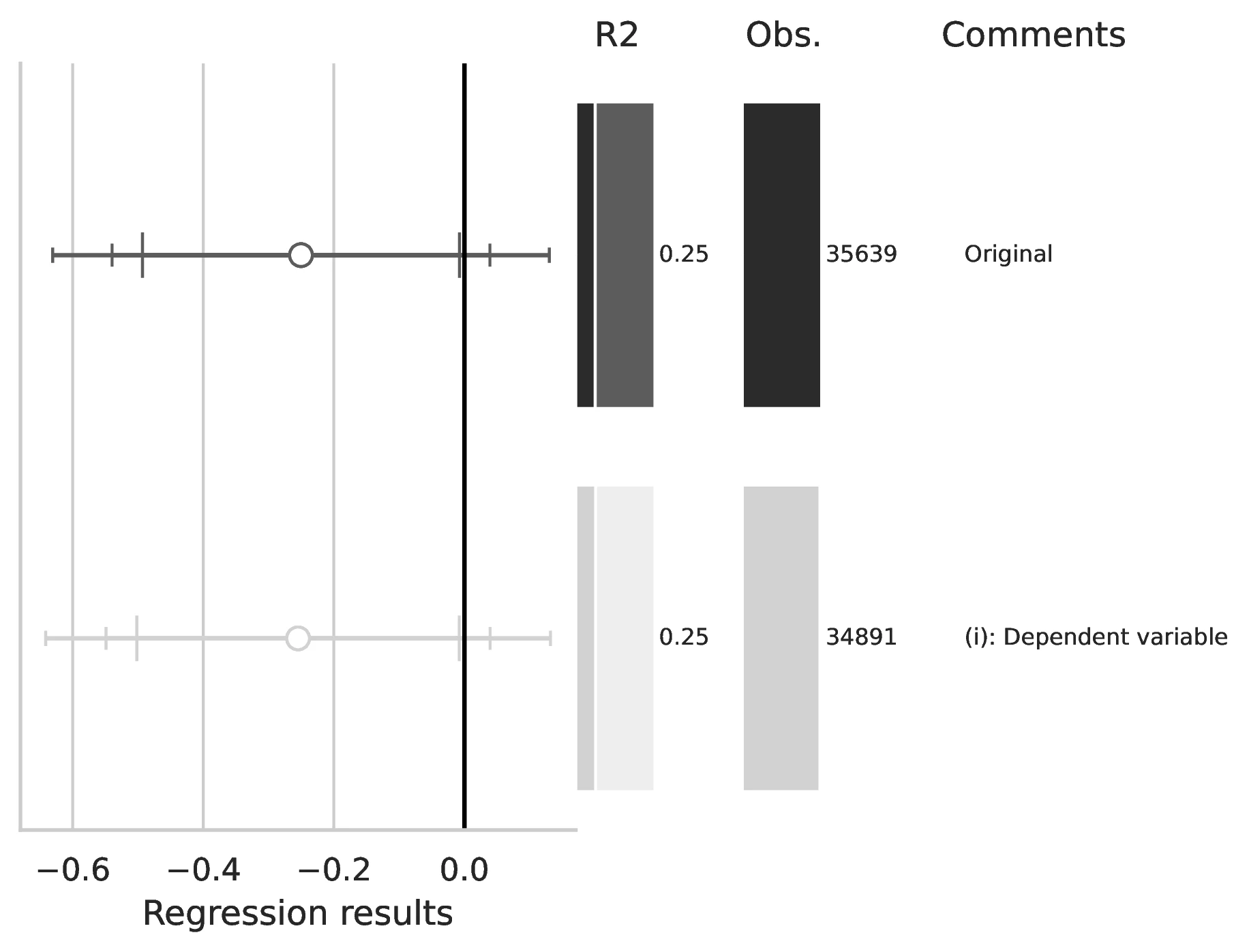
Notes: This figure compares the original estimation (black) with the corrected results (gray) for Equation 4, originally reported in Table 4 of GN. The graphical representation focuses on the main coefficient of interest in each column (interaction term where applicable), and includes confidence intervals, sample size, and \(R^2\), with comments on the corrections implemented.
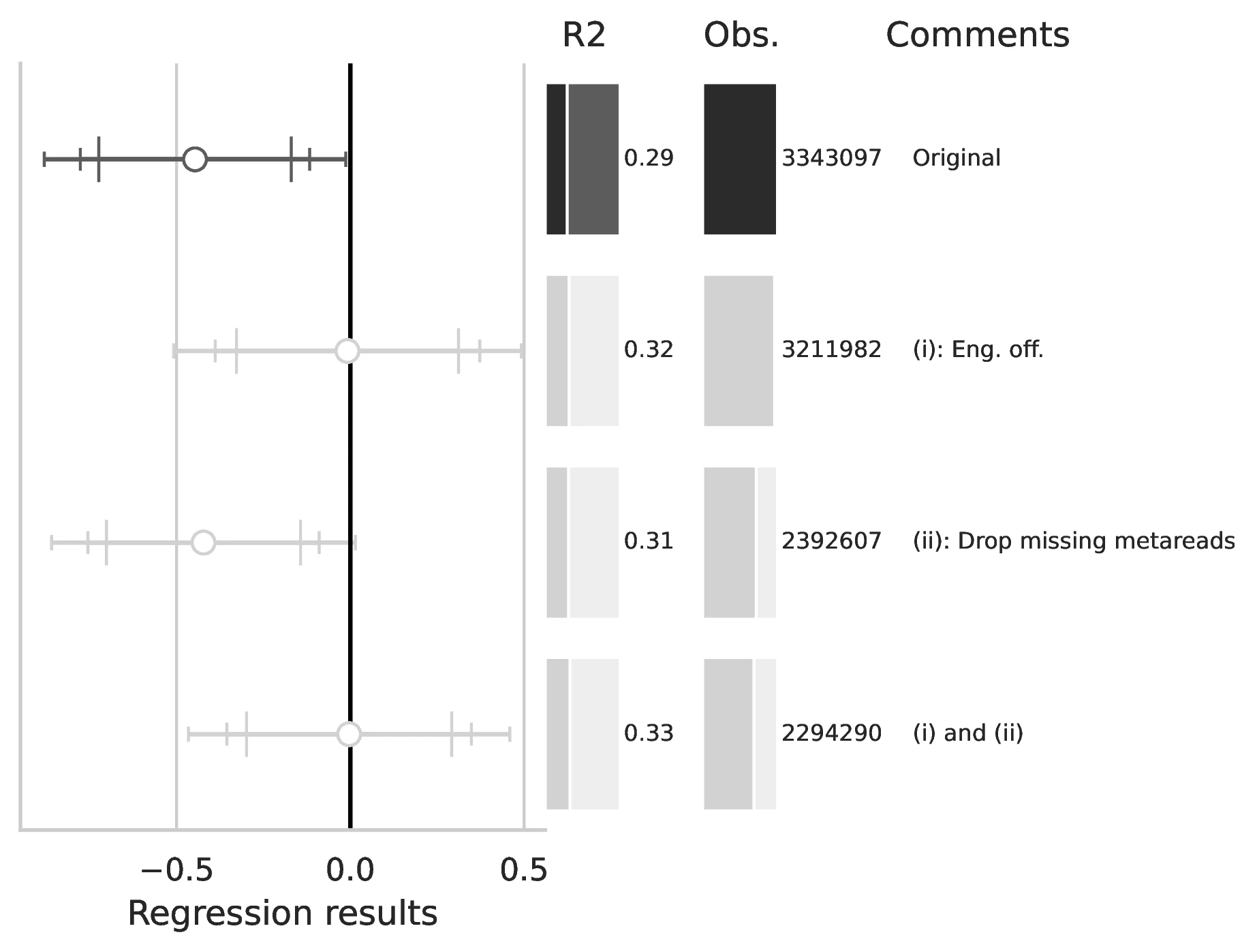

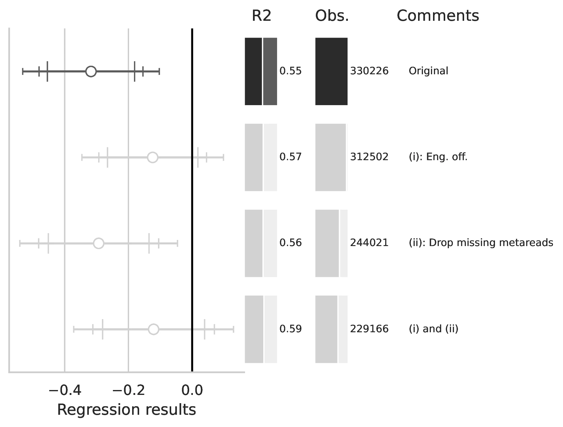

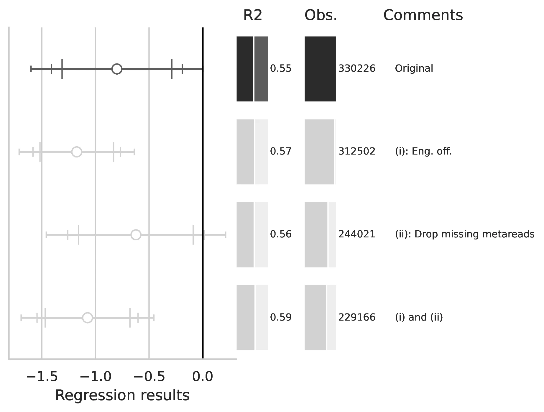
Notes: This figure compares the original estimation (black) with the corrected results (gray) for Equation 5 and Equation 6, originally reported in Table 5 of GN. The graphical representation focuses on the main coefficient of interest in each column (interaction term where applicable), and includes confidence intervals, sample size, and \(R^2\), with comments on the corrections implemented.
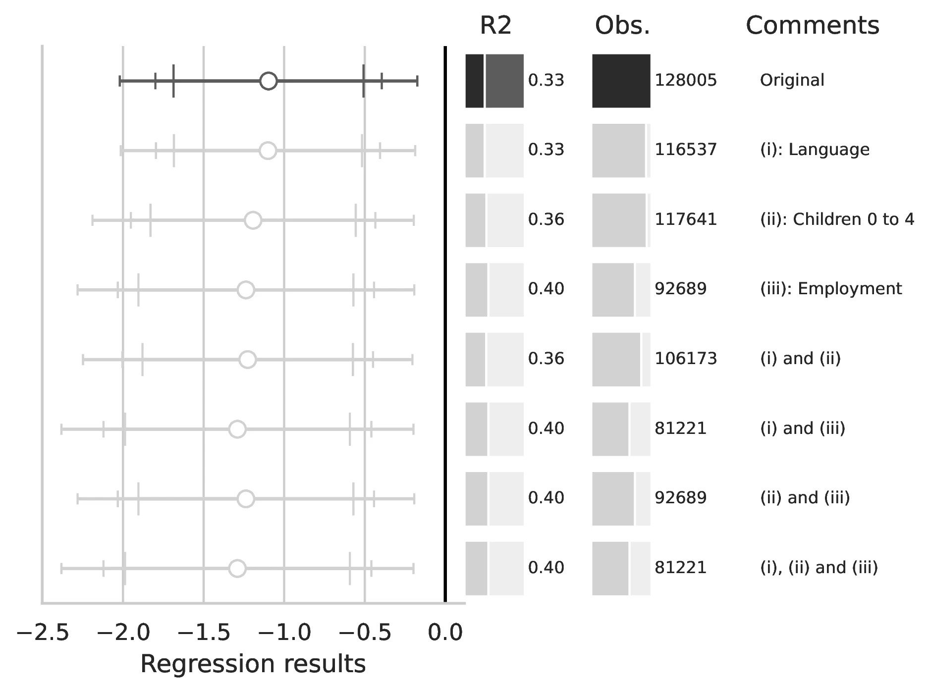
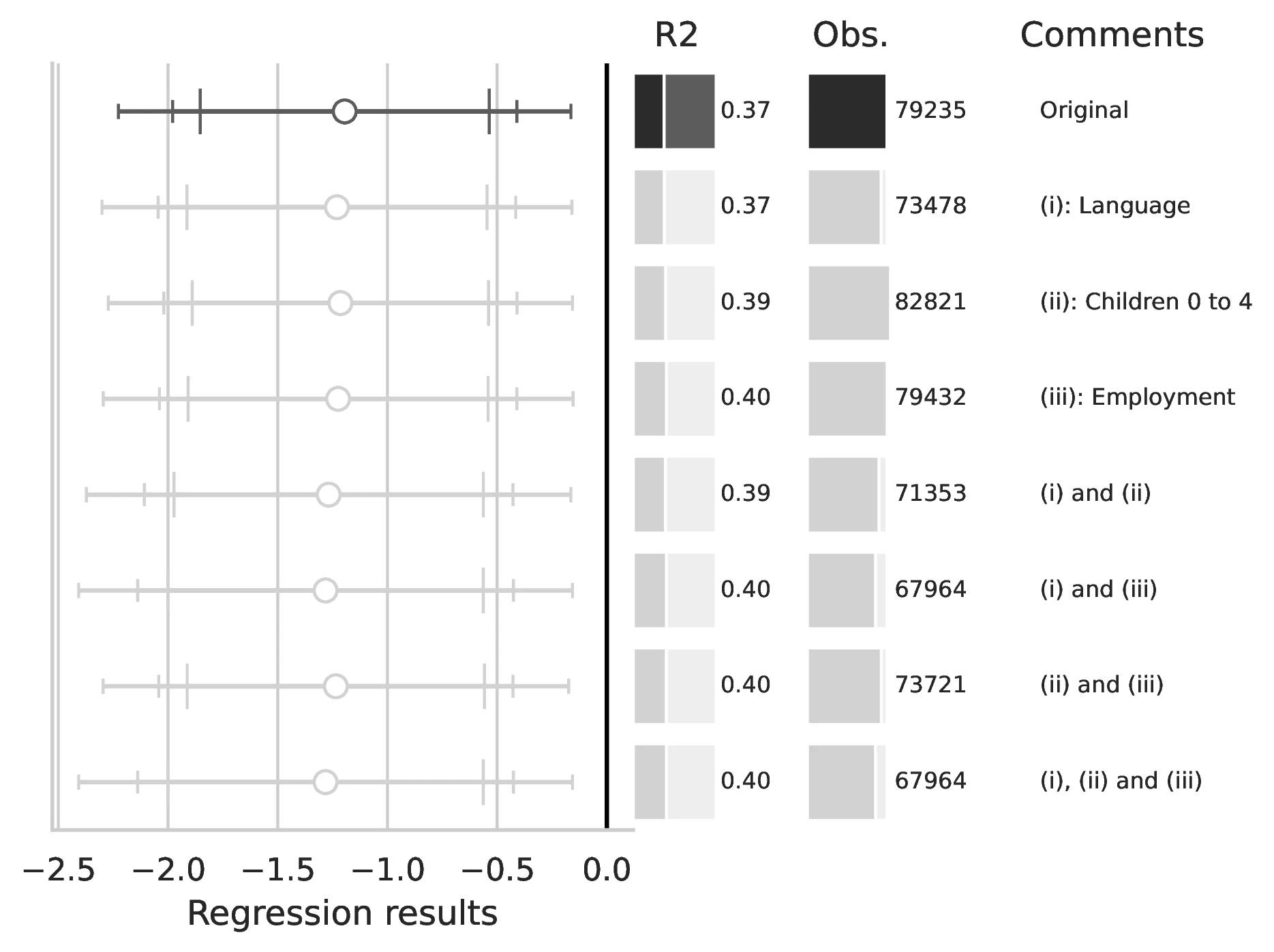
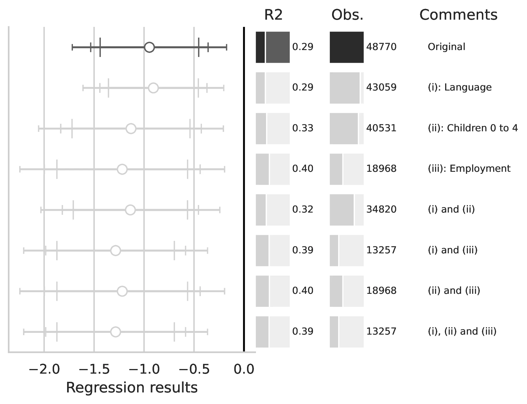
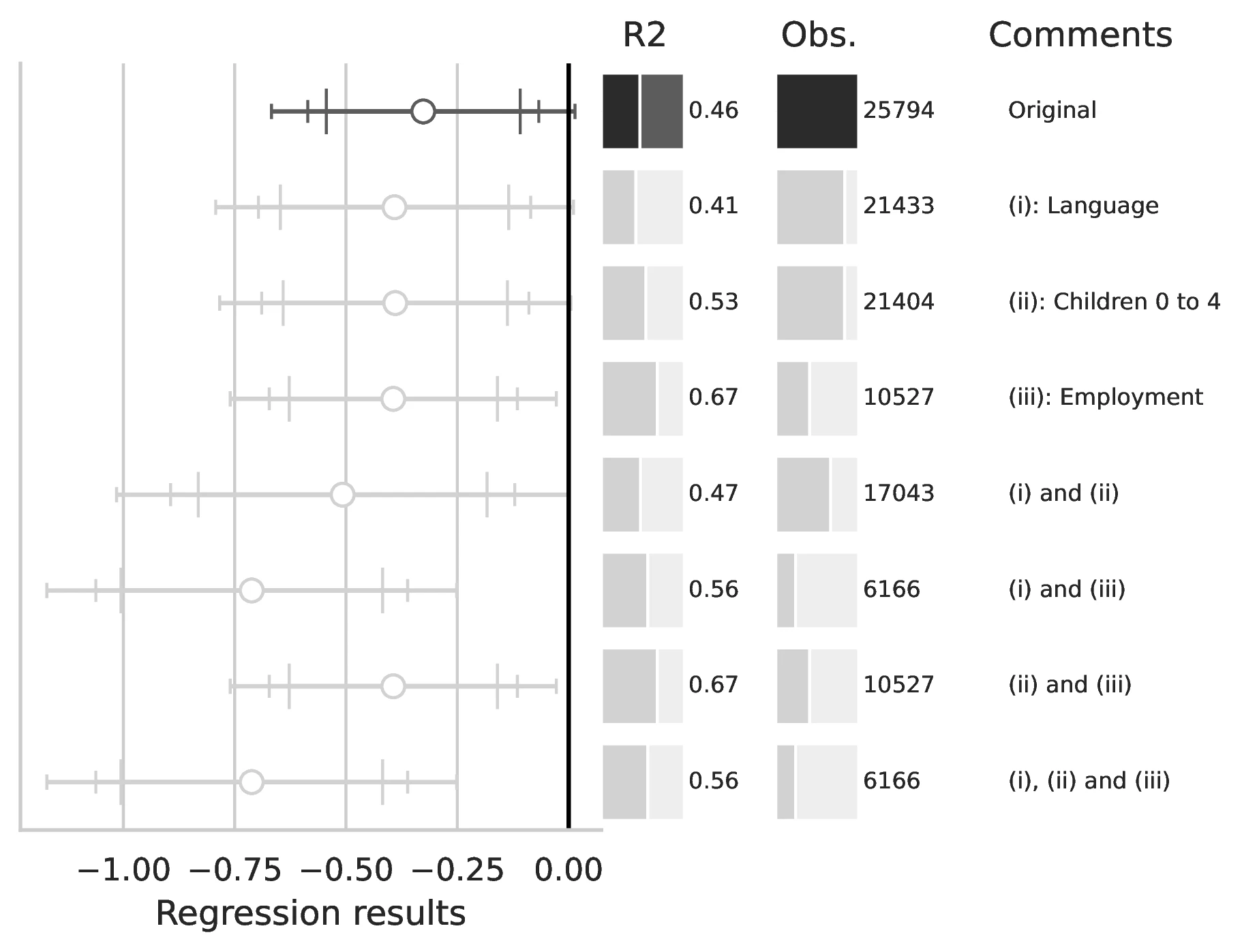
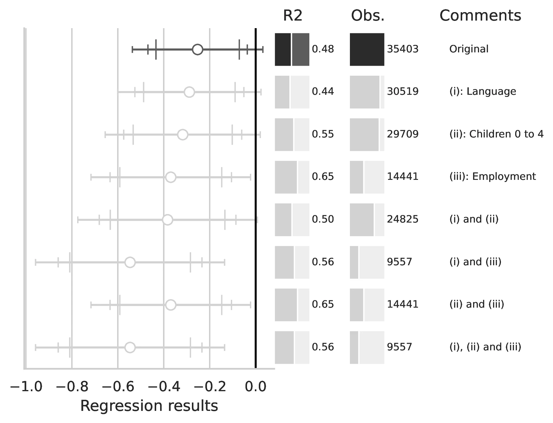

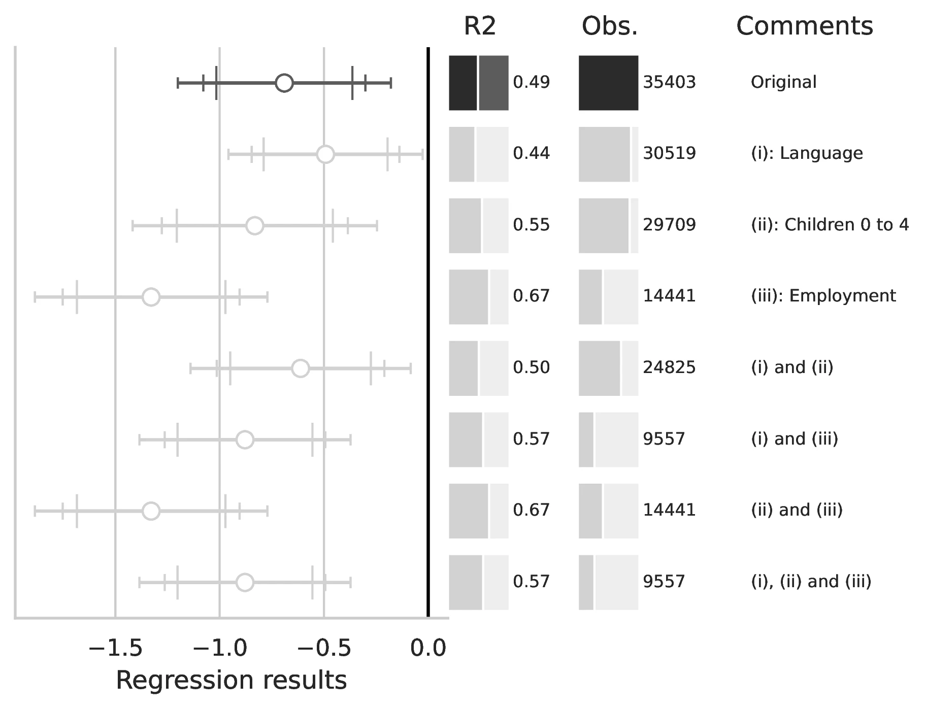
Notes: This figure compares the original estimation (black) with the corrected results (gray) for Equation 8 and Equation 9, originally reported in Table 7 of GN. The graphical representation focuses on the main coefficient of interest in each column (interaction term where applicable), and includes confidence intervals, sample size, and \(R^2\), with comments on the corrections implemented.
3 Concluding remarks
Our “deep reproduction” of the individual-level analysis from the study by Giuliano and Nunn (2021) was unsuccessful. Despite the Authors’ corrigendum (Giuliano and Nunn 2024), which addresses some imprecision in the original text, we identified several remaining discrepancies between the precise descriptions provided in the article and the corresponding code included in the replication package. These inconsistencies span multiple aspects of the analysis, including variable definitions, sample selection criteria, and regression specifications. Our exercise suggests that correcting for these inconsistencies has a significant impact on the results, which, upon re-examination, reveal a more nuanced relationship between ancestral climatic variability and tradition.
The deep reproduction exercise highlights the importance of ensuring consistency between the descriptions in published work and the underlying analysis code and data. Comprehensive replication packages, including all necessary files, can greatly facilitate verification efforts and enhance research transparency, and the steps taken in this direction by economic journals, such as the Review of Economic Studies, are clearly positive.
Appendices
| Eq. num | Inconsistency | Correction | Applied |
|---|---|---|---|
| 2 | The information used is not on mother tongue, but on the language that the respondent speaks at home | N/A | No |
| 4 | The dependent variable is defined only for individuals co-residing with their spouses | Exclude from the estimation sample observations for which the variable marst is equal to 2 (Married, spouse absent) | Yes |
| The control variable measuring “the fraction of the population in the same metropolitan area as the individual who are first or second-generation immigrants from the same country of origin” (p. 1562) is computed separately for each year from 1994 to 2014 | Compute the variable in a time-invariant way | No | |
| The “natural log of the current per-capita GDP in the country of origin (measured in the survey year)” is entirely missing for the year 2014 | Add the GPD data for 2014 | No | |
| The estimation samples include individuals that reside in metropolitan areas that are not separately identified (i.e. “Other metropolitan areas, unidentified”; “NIU, household not in a metropolitan area”; “Missing data”) | Exclude observations for which the variable metarea is equal to 9997, 9998 and 9999 |
Yes | |
| The control variable measuring “the fraction of the population in the same metropolitan area as the individual who are first or second-generation immigrants from the same country of origin” (p. 1562) is not constant, for individuals associated to the same foreign country \(c\), surveyed in the same year | The control variable should be defined in a way that does not vary, when the variable metarea is equal to 9997, 9998 or 9999, across observations corresponding to a unique value of \(c\) | No | |
| 5–6 | The value of the variable lingprox_dominant_a associated with Canada corresponds to English and stands at 15. However, the estimation sample excludes natives of Canadian ancestry, but includes natives of French Canadian ancestry |
Exclude observations for which isocode is “CAN” or replace the value of lingprox_dominant_a by the one corresponding to French (1) | Yes |
| The estimation sample include individuals that reside in metropolitan areas that are not separately identified (i.e. “Not identifiable or not in an MSA”) | Exclude observation for which he variable metarea is equal to 0 | Yes | |
| The variable measuring the “fraction of those living in the same metropolitan area who are first-generation immigrants of the same ancestry” (p. 1565) is incorrectly defined for the observations for which the variable metaread is equal to 0. | Exclude observation for which the variable metarea is equal to 0 | Yes | |
| The split between living and not living with parents is done using the variable relate, which only describes the relationship of individual \(i\) to the household head | Use the variables momloc and poploc, available from IPUMS USA (Ruggles et al., 2023). |
No | |
| 8–9 | The questionnaire of the 1930 census did not include the two questions necessary to define the dependent variable | Exclude the observations drawn from the 1930 census | Yes |
| The two questions necessary to define the dependent variable are asked to individuals aged 5 and above | Exclude the observations for children aged 0 to 4 | Yes | |
| The question necessary to define the employment status is asked to individuals aged 16 and above | Exclude the observations for children aged 0 to 15 | Yes | |
| The estimation sample include individuals that reside in metropolitan areas that are not separately identified (i.e. “Not identifiable or not in an MSA”). | Exclude observation for which the variable metarea is equal to 0. |
Yes | |
The split between living and not living with parents is done using the variable relate, which only describes the relationship of individual i to the household head |
Use the variables momloc and poploc, available from IPUMS USA (Ruggles et al., 2023) |
No |
Notes: Summary of the corrections.
| Table number | Column number | Equation number | |
|---|---|---|---|
| A25 | 1-5 | 8 | |
| 6 | 10 | ||
| A26 | 1-5 | 8 | |
| A27 | 1-5 | 8 | |
| A30 | 1-5 | 8 | |
| A31 | 1-5 | 8 |
Notes: This tables describes the errors in the original appendix.
| Dependant variable: indicator variable for spouse being from the same origin country | ||||
|---|---|---|---|---|
| Sample | Married women | Married men | ||
| Origin country identified from | Father | Mother | Father | Mother |
| (1) | (2) | (3) | (4) | |
| Climatic instability | -0.278* | -0.489*** | -0.107 | -0.255* |
| (0.155) | (0.178) | (0.140) | (0.150) | |
| Country-level controls: | ||||
| Distance from equator | -0.006** | -0.005 | -0.008*** | -0.009*** |
| (0.003) | (0.003) | (0.003) | (0.003) | |
| Economic complexity | 0.006 | 0.015 | -0.013 | -0.023 |
| (0.028) | (0.037) | (0.040) | (0.039) | |
| Political hierarchies | 0.094*** | 0.088*** | 0.094** | 0.088** |
| (0.028) | (0.030) | (0.038) | (0.039) | |
| Ln (per capita GDP) | -0.002 | -0.019 | -0.001 | -0.003 |
| (0.031) | (0.035) | (0.037) | (0.036) | |
| Genetic distance from the US | 0.030 | 0.009 | 0.012 | -0.008 |
| (0.047) | (0.055) | (0.045) | (0.046) | |
| Fraction of population in location who | 3.405*** | 3.622*** | 3.104*** | 3.430*** |
| are 1st or 2nd-generation immigrants | (0.509) | (0.655) | (0.520) | (0.503) |
| from same country of origin | ||||
| Individual controls | Yes | Yes | Yes | Yes |
| Number of countries | 108 | 105 | 110 | 105 |
| Mean (st.dev.) of dependent variable | 0.33 (0.47) | 0.32 (0.47) | 0.28 (0.45) | 0.29 (0.45) |
| Observations | 35,075 | 33,083 | 37,641 | 34,891 |
| Original observations | 36,082 | 34,045 | 38,419 | 35,639 |
| \(R^{2}\) | 0.251 | 0.267 | 0.228 | 0.251 |
Notes: Mistake (Dependent variable) is corrected. Mistake (Missing MSA 1) is not corrected. Mistakes (Fraction of the population) and (GDP 2014) cannot be corrected. Except for these corrections, the specification is strictly the same as in GN.
| Dependant variable: indicator variable for spouse being from the same origin country | ||||
|---|---|---|---|---|
| Sample | Married women | Married men | ||
| Origin country identified from | Father | Mother | Father | Mother |
| (1) | (2) | (3) | (4) | |
| Climatic instability | -0.330* | -0.528** | -0.146 | -0.294* |
| (0.194) | (0.209) | (0.166) | (0.176) | |
| Country-level controls: | ||||
| Distance from equator | -0.006** | -0.005 | -0.008** | -0.009*** |
| (0.003) | (0.003) | (0.003) | (0.003) | |
| Economic complexity | 0.008 | 0.014 | -0.015 | -0.021 |
| (0.029) | (0.037) | (0.043) | (0.041) | |
| Political hierarchies | 0.094*** | 0.088*** | 0.095** | 0.091** |
| (0.029) | (0.031) | (0.040) | (0.039) | |
| Ln (per capita GDP) | -0.007 | -0.023 | -0.002 | -0.006 |
| (0.033) | (0.036) | (0.040) | (0.038) | |
| Genetic distance from the US | 0.017 | -0.002 | 0.007 | -0.017 |
| (0.048) | (0.054) | (0.047) | (0.046) | |
| Fraction of population in location who | 3.321*** | 3.564*** | 2.938*** | 3.244*** |
| are 1st or 2nd-generation immigrants | (0.515) | (0.644) | (0.558) | (0.530) |
| from same country of origin | ||||
| Individual controls | Yes | Yes | Yes | Yes |
| Number of countries | 106 | 105 | 110 | 105 |
| Mean (st.dev.) of dependent variable | 0.35 (0.48) | 0.34 (0.48) | 0.31 (0.46) | 0.31 (0.46) |
| Observations | 28,860 | 27,427 | 30,413 | 28,342 |
| Original observations | 36,082 | 34,045 | 38,419 | 35,639 |
| \(R^{2}\) | 0.250 | 0.263 | 0.229 | 0.249 |
Notes: Mistakes (Dependent variable) and (Missing MSA 1) are corrected. Mistakes (Fraction of the population) and (GDP 2014) cannot be corrected. Except for these corrections, the specification is strictly the same as in GN.
| Dep. variable: Indicator for speaking an Indigenous language at home | |||||||
| All 2nd gen+ individuals | Not living with parents | Living with parents | |||||
| (1) | (2) | (3) | (4) | (5) | (6) | (7) | |
| Climatic instability | -0.003 | 0.055 | -0.427** | -0.121 | -0.131 | 0.132 | 0.125 |
| (0.179) | (0.192) | (0.214) | (0.097) | (0.098) | (0.084) | (0.083) | |
| Father speaks a foreign language | 0.503*** | 0.791*** | |||||
| (0.029) | (0.058) | ||||||
| Mother speaks foreign lang.\(\times\) Climatic instability | -1.074*** | ||||||
| (0.240) | |||||||
| Mother speaks a foreign language | 0.511*** | 0.809*** | |||||
| (0.030) | (0.056) | ||||||
| Father speaks foreign lang.\(\times\) Climatic instability | -1.102*** | ||||||
| (0.225) | |||||||
| Individual controls | Yes | Yes | Yes | Yes | Yes | Yes | Yes |
| Number of countries | 77 | 77 | 77 | 77 | 77 | 77 | 77 |
| Mean (st.dev.) of dependent variable | 0.13 (0.34) | 0.11 (0.32) | 0.25 (0.43) | 0.25 (0.43) | 0.25 (0.43) | 0.25 (0.43) | 0.25 (0.43) |
| Observations | 2,294,290 | 1,994,785 | 299,505 | 229,166 | 280,396 | 229,166 | 280,396 |
| Original observations | 3,343,097 | 2,915,673 | 427,424 | 330,226 | 400,062 | 330,226 | 400,062 |
| \(R^{2}\) | 0.332 | 0.298 | 0.420 | 0.588 | 0.602 | 0.592 | 0.606 |
Notes: Mistakes (Missing MSA 2) and (English) are corrected. Mistake (Living with parents) cannot be corrected. Except for these corrections, the specification is strictly the same as in GN.
| Dep. variable: Indicator for speaking a foreign language at home | |||||||
| All 2nd gen+ individuals | Not living with parents | Living with parents | |||||
| (1) | (2) | (3) | (4) | (5) | (6) | (7) | |
| Climatic instability | -1.290*** | -1.282*** | -1.284*** | -0.712*** | -0.547*** | -0.356** | -0.193 |
| (0.424) | (0.437) | (0.357) | (0.179) | (0.160) | (0.152) | (0.149) | |
| Father speaks an Indigenous language | 0.448*** | 0.677*** | |||||
| (0.051) | (0.063) | ||||||
| Father speaks an Indigenous lang.\(\times\) Climatic instability | -0.902*** | ||||||
| (0.169) | |||||||
| Mother speaks an Indigenous language | 0.471*** | 0.694*** | |||||
| (0.046) | (0.051) | ||||||
| Mother speaks an Indigenous lang.\(\times\) Climatic instability | -0.878*** | ||||||
| (0.196) | |||||||
| Individual controls | Yes | Yes | Yes | Yes | Yes | Yes | Yes |
| Number of ethnic groups | 19 | 19 | 19 | 19 | 19 | 19 | 19 |
| Number of clusters (grid cells) | 18 | 18 | 18 | 18 | 18 | 18 | 18 |
| Mean (st.dev.) of dependent variable | 0.21 (0.41) | 0.21 (0.41) | 0.23 (0.42) | 0.31 ( 0.46) | 0.29 (0.46) | 0.31 (0.46) | 0.29 (0.46) |
| Observations | 81,221 | 67,964 | 13,257 | 6,166 | 9,557 | 6,166 | 9,557 |
| Original observations | 128,005 | 79,235 | 48,770 | 25,794 | 35,403 | 25,794 | 35,403 |
| \(R^{2}\) | 0.396 | 0.399 | 0.395 | 0.557 | 0.564 | 0.564 | 0.570 |
Notes: Mistakes (Language), (Children 0 to 4) and (Employment) are corrected. Mistake (Missing MSA) is not corrected. Mistake (Living with parents) cannot be corrected. Except for these corrections, the specification is strictly the same as in GN.
| Dep. variable: Indicator for speaking a foreign language at home | |||||||
| All 2nd gen+ individuals | Not living with parents | Living with parents | |||||
| (1) | (2) | (3) | (4) | (5) | (6) | (7) | |
| Climatic instability | -0.364 | -0.380 | -0.140 | -0.172 | 0.064 | 0.040 | 0.107 |
| (0.268) | (0.275) | (0.191) | (0.116) | (0.072) | (0.095) | (0.093) | |
| Father speaks an Indigenous language | 0.362*** | 0.628*** | |||||
| (0.062) | (0.097) | ||||||
| Father speaks an Indigenous lang.\(\times\) Climatic instability | -1.041** | ||||||
| (0.483) | |||||||
| Mother speaks an Indigenous language | 0.408*** | 0.456*** | |||||
| (0.058) | (0.110) | ||||||
| Mother speaks an Indigenous lang.\(\times\) Climatic instability | -0.185 | ||||||
| (0.438) | |||||||
| Individual controls | Yes | Yes | Yes | Yes | Yes | Yes | Yes |
| Number of ethnic groups | 19 | 19 | 19 | 18 | 19 | 18 | 19 |
| Number of clusters (grid cells) | 18 | 18 | 18 | 17 | 18 | 17 | 18 |
| Mean (st.dev.) of dependent variable | 0.10 (0.30) | 0.10 (0.31) | 0.09 (0.29) | 0.15 (0.35) | 0.13 (0.34) | 0.15 (0.35) | 0.13 (0.34) |
| Observations | 34,092 | 29,500 | 4,592 | 1,791 | 2,903 | 1,791 | 2,903 |
| Original observations | 128,005 | 79,235 | 48,770 | 25,794 | 35,403 | 25,794 | 35,403 |
| \(R^{2}\) | 0.381 | 0.386 | 0.416 | 0.533 | 0.562 | 0.542 | 0.562 |
Notes: Mistakes (Language), (Children 0 to 4), (Employment) and (Missing MSA) are corrected. Mistake (Living with parents) cannot be corrected. Except for these corrections, the specification is strictly the same as in GN.
References
Footnotes
In this way, GN overcome the challenges arising from the correlation between historical and current climatic variability. The literature on the determinants of culture refers to this setup in which individuals from different origins residing in a single location are compared as the “epidemiological approach” (see Fernández 2011). We refer the reader to a companion paper (Bertoli et al. 2023) which discusses the analytical challenges related to the use of self-reported ancestry to identify the foreign countries of origin of natives, as GN do in a portion of their work.↩︎
The literature on persistence and rapid cultural change is vast and multifaceted. For a comprehensive overview, see Bisin and Federico (2021); in particular, Voth (2021) provides a thorough survey of the persistence literature in historical economics, while Acemoglu et al. (2021) offers a conceptual framework for understanding institutional persistence and change. Empirical studies have also shed light on the dynamics of cultural change, such as Alesina and Fuchs-Schündeln (2007), which examines the effect of communism on people’s preferences, and Slotwinski and Stutzer (2022), which investigates the impact of religious doctrine on democratization.↩︎
Last version accessed: 30 November 2023.↩︎
We cite the earlier I4R Discussion Paper version of Dreber and Johannesson (2023), as requested by a referee, but the term “deep reproducibility” appears in a later version of the paper, posted on SSRN on May 25, 2023, and last revised on November 30, 2023, available at https://dx.doi.org/10.2139/ssrn.4458153.↩︎
The definition of “same” in the context of Clemens (2017) is crucial in our exercise: “[t]he ‘same’ specification, population, or sample means the same as reported in the original paper, not necessarily what was contained in the code and data used by the original paper. Thus for example if code used in the original paper contains an error such that it does not run exactly the regressions that the original paper said it does, new code that fixes the error is nevertheless using the ‘same’ specifications (as described in the paper).” (p. 328).↩︎
We successfully verified the computational reproducibility of the results in GN for which the code is included.↩︎
Giuliano and Nunn (2024) acknowledges our contribution to this corrigendum.↩︎
It should be noted, however, that there are instances where it is possible to infer inconsistencies between the original article’s text and the analysis code, particularly when the aggregate data is directly linked to underlying individual-level data used in other equations. For example, coding errors in the generation of the dependent variable in Eq. (8) extend to Eq. (10), as the latter equation simply aggregates the individual-level data used to estimate the former (see Tables 8 and 10). Additionally, the final point of the corrigendum (Giuliano and Nunn 2024) addresses an inconsistency between the original article’s text and the corresponding analysis code using aggregate data.↩︎
Regressions using indigenous population are similarly regarded. Eq. (2) uses individual-level data but only compares “individuals living in the same country but belonging to different ethnic groups." (Giuliano and Nunn 2021, 1543)↩︎
We refer the reader to Table [tab:synthesis] in the online Appendix for a summary of the identified inconsistencies, the corrections we propose and whether we implemented them or not. This Table also associates each inconsistency to the equation in which it appears. Table 1 indicates the Tables and Columns with errors in the original Appendix, together with the equations that these estimated.↩︎
For instance, we mention that cohabiting parents and children could be identified using the variables
poplocandmomloc. These variables are not included in the replication package, and since individual identifiers have been removed, it is impossible to merge the data from the replication package with the original information from IPUMS.↩︎For the reader’s interest, our online Appendix presents the results obtained when we simultaneously correct all feasible discrepancies. Additionally, Figure 1–Figure 3 illustrate the estimates obtained when addressing different combinations of these discrepancies. These figures serve to evaluate the impact of resolving various issues on the estimated coefficient of the variable of interest.↩︎
Equation 2 is estimated in the six data columns of Table 2; Equation 4 is estimated in the four data columns of Table 4; Equation 5 in Cols. (1)-(5) in Table 5; Equation 6 in Cols. (6) and (7) in Table 5; Equation 8 in Cols. (1)-(5) in Table 7, and Equation 9 in Cols. (6) and (7) in Table 7.↩︎
We do not provide corrections for Equation 2, because the code that exactly follows the description given in the original article is impossible to estimate, as a variable is simply not available in the data, and because the corrigendum realigns the text with the corresponding code.↩︎
The actual incidence depends on the (unobserved) share of each estimation sample for which the mother tongue is not the language normally spoken at home.↩︎
“Since children born to immigrant parents in the U.S. are almost always fluent in English, they face the decision of whether to continue speaking their traditional language at home. They face this decision both when they live with their parents as children and when they live on their own with their own family. Thus, as a revealed measure of the importance of maintaining tradition, we examine the extent to which a foreign language is spoken at home among the children of immigrants. Speaking a foreign language at home indicates that the children of the immigrants were taught their origin language, which is a sign of the parents and children valuing their tradition.” (p. 1565).↩︎
See, for instance, User Note 1 in Appendix G of the Codebook of the 1994 March Supplement of the CPS, available at: https://cps.ipums.org/cps/resources/codebooks/cpsmarapr94.pdf (last accessed: June 25, 2023).↩︎
For each equation, the incidence have been computed by dividing the number of observations corresponding to countries with a non-missing GDP in 2013, but a missing GDP in 2014 and all other variables that are non-missing, by the total number of observations in the sample↩︎
This variable is also entirely missing for some countries of origin (e.g., Argentina, Syria), leading to their exclusion from the estimation. However, the exact same control variable exists for these countries for the year 2000 in Equation 5 and Equation 6.↩︎
The seven countries or territories are Canada, Puerto Rico, the Philippines, India, Samoa, Pakistan, and Eritrea; we identify countries and territories where English is an official language by cross-checking Wikipedia contributors (2023) and Central Intelligence Agency (2021), retaining only the cases in which both data sources report English as an official language.↩︎
The replication package includes the three-digit ISO code of the country of ancestry, not the name of the ancestral group.↩︎
Notice that the linguistic proximity between the United States and France (French) is 1; the only other country of ancestry with a value of 15 (the value corresponding to English) is Samoa, which is also a country with English as an official language, and the second highest value is 8 (for Puerto Rico), a territory with English as an official language, and the average linguistic proximity stands at 2.2 in the Authors’ original sample; this contributes to explain why the limited share of observations corresponding to countries where English is an official language play such a pivotal role in the significance of the variable of interest.↩︎
“In columns 2 and 3, we split the samples into those not living with their parents and those living with their parents.” (p. 1567).↩︎
These variables provide the identifiers of the co-residing mother and father. See, for instance, https://usa.ipums.org/usa-action/variables/MOMLOC#availability_section (last accessed on May 31, 2023). Using these variables also avoids incorrectly identifying a step-father as the father of the child, something that may occur using
relate.↩︎See https://usa.ipums.org/usa-action/variables/LANGUAGE#availability_section (last accessed on May 31, 2023).↩︎
See https://usa.ipums.org/usa-action/revisions#revision_02_09_2021 (last accessed on October 23, 2023); we thank Paola Giuliano and Nathan Nunn for bringing this to our attention.↩︎
See https://usa.ipums.org/usa-action/variables/MTONGUE#description_section (last accessed on October 23, 2023).↩︎
Private communication with Paola Giuliano and Nathan Nunn, who contacted IPUMS USA for clarification.↩︎
The share of observations where the dependent variable equals 1 is 91.0 for Navajo and 99.2 percent for Hopi in 1930.↩︎
It is worth noting that the replication package only includes the binary dependent variable and does not provide information on the language associated with each individual.↩︎
See https://usa.ipums.org/usa-action/variables/LANGUAGE#universe_section (last accessed on June 6, 2023).↩︎
See https://usa.ipums.org/usa-action/variables/EMPSTAT#universe_section (last accessed on October 23, 2023).↩︎
These two tables differ in their treatment of observations with a missing metropolitan area. The former includes those while the latter does not.↩︎
Similarly to Table 4, we present two variants of Table 7. The first includes observations with a missing metropolitan area. The second does not.↩︎
Reuse
Citation
@online{bertoli2024,
  author = {Bertoli, Simone and Clerc, Melchior and Loper, Jordan and
    Roca Fernández, Èric},
  title = {Understanding Cultural Persistence and Change: A Replication
    of {Giuliano} and {Nunn} (2021)},
  date = {2024-07-18},
  doi = {10.1111/ecin.13242},
  langid = {en},
  abstract = {Giuliano and Nunn (2021) provide econometric evidence that
    ancestral climatic variability reduces the current importance of
    tradition. We conduct a “deep reproduction”, comparing the precise
    descriptions of the individual-level regressions in their article
    with the corresponding code. This analysis uncovers several major
    inconsistencies, also related to the code not included in their
    replication package. A published *corrigendum* addresses some
    inconsistencies we had also communicated to the Editor of REStud,
    but several remain, relating to a substantial portion of the
    observations. A realignment of the code with the text reveals a more
    nuanced relationship between ancestral climatic variability and
    tradition.}
}