Changes in $G$

We focus now on how a change in $G_{t}$ affects the behaviour of the economy. We rely on the phase diagram for this analysis: it conveys the message quite efficiently. In what follows, we assume that the economy is at its steady-state level $(\bar{k}^{\mathcal{Gov}}, \bar{c}^{\mathcal{Gov}})$ when the government decides to change $G_t.$ Furthermore, we assume taxes are constant at some level $G_{t} = G_{1} > 0.$

Unexpected, permanent rise in $G$

Suppose that the government announces a sudden and unexpected increase in $G: G_{2} > G_{1}.$ The Ramsey model illustrates the consequences of such a change.

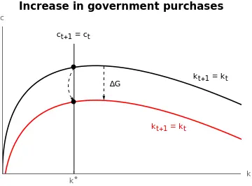
First, we assumed that the economy was at its steady state. The change in $G$, as we discussed before, moves the $k$-locus closer to the horizontal axis.

With the change in $G$, a new steady state emerges. The steady-state capital level $\bar{k}^\mathcal{Gov}(G_2) = \bar{k}^\mathcal{Gov}(G_{1})$ remains the same. However, households need to adjust their consumption level. Otherwise, they would not be on the saddle path, and they would follow a diverging trajectory leading to zero consumption. The unique possibility that puts the economy in the new steady state is for consumption to jump directly into it. This is, consumption must be reduced by the amount $\Delta_{G} = G_{2} - G_{1}.$ Thus the size of the immediate fall in consumption is equal to the full amount of the increase in government purchases, and the capital stock and the real interest rate are unaffected.

A similar policy under the Solow model would have implied a smaller reduction in consumption. In Solow, consumption is the fraction $1-s$ of current income. The tax decreases current income by $G$, but consumption would only change by $(1-s)G < G.$ Hence, the remaining part of the increase in $G$ is absorbed by a reduction in investments of the size $sG$: government purchases crowd out investment in the Solow model.

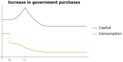
Unexpected, temporary rise in $G$

Different from before, suppose that the increase in $G$ is only temporary, starting at $t=t_{0}$ and lasting until $t=t_{1}.$ We still suppose that the increase in taxes is unexpected. One possibility is to first jump to the new steady state, remain there while taxes are high, and at time $t=t_{1}$ jump back to the original steady state. However, this implies two discontinuities in consumption: the first and second jumps. This would imply that marginal utility falls discontinuously and this is not optimal.

There is a second possibility. First, decrease consumption by a smaller amount than before: $\Delta_{c} < \Delta_{G}.$ This implies that the economy is not in the new steady state $(\bar{k}^\mathcal{Gov}(G_2) , \bar{c}^{\mathcal{Gov}}(G_{2}))$, but above it. Thus, it is subject to the dynamics implied by the phase diagram: capital decreases and consumption increases. The initial jump in consumption must be carefully computed such that, at time $t=t_{1}$, the dynamics implied by $G_{2}$ put the economy on the saddle path of $G_{1}.$ This is, the economy undergoes a transition such that, at $t=t_{1}$ when taxes and dynamics —and the phase diagram— return to the original configuration, the economy is on its saddle path.

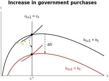
The figure above depicts in black the original $k$-locus —for $G=G_{1}$— and in red the temporary one while with $G=G_{2}.$ The economy first jumps from the initial steady state $(\bar{k}^{\mathcal{Gov}}(G_{1}), \bar{c}^{\mathcal{Gov}}(G_{1}))$ following the black arrow. From then onwards, the dynamics of the red $k$-locus determine the trajectory of the economy. In particular, it moves north-west following the orange curve. The initial jump is calculated in such a way that at $t=t_{1}$ the economy is on the saddle path corresponding to $G=G_{1}.$ From there, it simply follows the saddle path towards the steady state $(\bar{k}^{\mathcal{Gov}}(G_{1}), \bar{c}^{\mathcal{Gov}}(G_{1})).$

During the transition, households reduce capital to sustain a higher and increasing level of consumption that would not be possible with $G_{2} > G_{1}.$ From $t=t_{1}$, consumption continues to grow, but capital starts accumulating again.

The change in consumption during $t=t_{0}$ is directly proportional to the length of the increase in taxes. The longer it is, the closer the economy jumps to the steady state $(\bar{k}^{\mathcal{Gov}}(G_{2}), \bar{c}^{\mathcal{Gov}}(G_{2})).$ However, it never reaches it: households always decrease their savings, which allows them to later be on the saddle path when taxes go back to $G_{1}.$

Anticipated, permanent rise in $G$

Note: when analysing an anticipated measure, start from the end move backwards.

Suppose that at time $t=t_{0}$ the government announces that at time $t=t_{1}$ taxes will permanently increase.

One possibility is to mimic the [unanticipated, permanent change](<{{ ref “#un_perm” >}}): remain at the original steady state $(\bar{k}^\mathcal{Gov}(G_{0}), \bar{c}^\mathcal{Gov}(G_{0}))$ until $t_{1}$, and then jump onto the new steady state. However, this represents a large cost in terms of utility: non-smooth changes penalise utility.

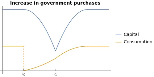
Instead, households will slightly decrease consumption at $t_{0}$. The dynamics of the $(\bar{k}^\mathcal{Gov}(G_{0}), \bar{c}^\mathcal{Gov}(G_{0}))$ steady state will move the economy south-east: consumption decreases while capital increases. The first initial jump at $t_{0}$ must be such that, at $t_{1}$ the economy is on the saddle path corresponding to the new steady state $(\bar{k}^\mathcal{Gov}(G_{1}), \bar{c}^\mathcal{Gov}(G_{1})).$

Hence, during the transition, consumption continuously falls, but smoothly. Capital, instead, first accumulates and decreases from $t_{1}$ onwards.

Anticipated, temporary rise in $G$

Note: when analysing an anticipated measure, start from the end move backwards.

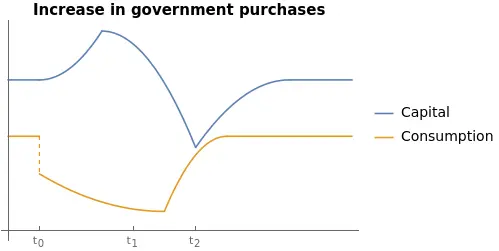
Finally, suppose that the increase in $G$ is temporary. At time $t=t_{0}$ the government announces that at time $t=t_{1}$ taxes will increase from $G_{0}$ to $G_{1}.$ The new tax regime will apply for some time, until $t=t_{2}$ when taxes will return to their original level $G_{0}.$

In that case households can decide to follow the same strategy as in an unanticipated, temporary increase. However, it entails a relatively large adjustment in terms of consumption at time $t=t_{1}$, when the new policy becomes effective. Instead, households can take advantage of the anticipation in the announcement: decrease the consumption at the announcement time $t=t_{0}$ by a relatively small amount. This places households on the black arrow trajectory, since the economy is still governed by the $(\bar{k}^\mathcal{Gov}(G_{0}), \bar{c}^\mathcal{Gov}(G_{0}))$-locus. In that case, though, the change in consumption is such that, when the new tax policy becomes effective, consumption follows the orange arrow. Finally, timing is again crucial because at time $t=t_{2}$ the economy must be on the saddle path that corresponds to the initial steady state: $(\bar{k}^\mathcal{Gov}(G_{0}), \bar{c}^\mathcal{Gov}(G_{0})).$

In that case, between $t_{0}$ and $t_{1}$, households decrease consumption and save. Between $t_{1}$ and $t_{2}$ first consumption continues to decrease and so does capital, but eventually consumption rises while capital continues to decrease. Finally, from $t_{2}$ onward, both capital and consumption rise along the saddle path. Note that, although consumption decreases, it does so continuously except for the initial jump. This consumption-smoothing decreases utility less than a discontinuous jumps.