Difference equations

This note is based on Appendix A.3.2 of de la Croix and Michel: A Theory of Economic Growth.

Macroeconomic models often have dynamic equations relating different periods of time. These can either be in continuous or discrete time. In this note, we focus only on the discrete-time case, but the intuition carries over to the continuous case. When equations are in discrete time, we call time difference equations. The continuous-time equivalents are called differential equations. Note: the conditions for stability change between the continuous and discrete-time cases.

A dynamic equation: one-dimensional case

A dynamic equation is an equation that relates the state of a variable through time to the value the variable took in previous periods. The number of lags the equation considers determines its order. A difference equation of order $T$ takes the form $$x_{t+1} = f(x_{t}, x_{t-1}, \ldots, x_{t-T}).$$

First-order difference equation

One of the most common cases that arises in macroeconomic models is the first-order difference equation. It relates the present value of a variable to the value it took in the period immediately before:

$$x_{t+1} = f(x_{t}).$$

We are often interested in the steady state of difference equations. The steady state is defined as the set of values $\bar{x}$ (there can be more than one steady state) such that, if reached, the economy remains there. Equivalently, once reached, the value of the variable $x$ remains unchanged. Mathematically, $\bar{x}$ is a steady state of a first-order difference equation if

$$\bar{x} = f(\bar{x}).$$

Proving that a steady state $\bar{x}$ exists may involve using different techniques.

Example: Assume the following first-order difference equation:

$$x_{t+1} = x_{t}^{\eta} +\kappa, \kappa>0, \eta \in (0,1).$$

The steady state solves: $\bar{x} = \bar{x}^{\eta}+\kappa$.

To show that it exists we can prove that the function $F(\bar{x}) = \bar{x} - \bar{x}^{\eta} - \kappa$ as at least one root.
Note that $F(0) = -\kappa <0$ and that $\lim_{\bar{x} \rightarrow +\infty} F(\bar{x}) = + \infty.$ Hence, since it is a continuous function, it must have at least one solution. We can further show that it admits one and only one solution by proving that $x_{t+1}$ is a monotonous function of $x_{t}$. Monotonicity is the key here, not whether it increases or decreases, although in our case it is increasing.

$$\frac{\partial x_{t+1}}{\partial x_{t}} = \eta x_{t}^{\eta-1} > 0.$$

Hence, the function is monotonous (always increasing) and there is one and only one root.

Stability of a first-order difference equation

A steady state solution $\bar{x}$ to $\bar{x} = f(\bar{x})$ which is interior to the domain of $f$ is locally stable if for any initial value $x_{0}$ near enough to $\bar{x}$, the dynamics starting from $x_{0}$ converge to $\bar{x}$. In other terms, $$\lim_{t \rightarrow +\infty} x_{t} = \bar{x}.$$

To determine whether a steady state is stable we analyse whether the function converges towards that steady state. We typically use first-order conditions to determine the stability. However, these only apply to hyperbolic steady states.

Hyperbolic steady states

Assume that $f$ is differentiable. Let $\bar{x}$ be a steady state of $f$.

• If $|f^{\prime}(\bar{x}) = 1|,$ then the steady state is non-hyperbolic.
• If $|f^{\prime}(\bar{x}) \neq 1|,$ then the steady state is hyperbolic.

First-order stability

Suppose that $\bar{x}$ is a hyperbolic steady state of $f$. Then

• if $|f^{\prime}(\bar{x})| < 1$ then $\bar{x}$ is locally stable,
• if $|f^{\prime}(\bar{x})| > 1$ then $\bar{x}$ is unstable.

Page 316 of de la Croix and Michel provides the proof.

Intuitively, the condition for stability requires that we approach the steady state slowly. In other terms, the curvature of $f$ is smaller than 1. Therefore, although $x_{t}$ grows over time, every time the increase in its value becomes smaller, eventually tending towards zero.

Example: let $x_{t} = f(x_{t-1}) = x_{t-1}^{0.5}$. This first-order difference equation has two steady states: $\bar{x}_{1} = 0$ and $\bar{x}_{2} = 1.$ The first derivative is $f^{\prime} = 0.5 x_{t-1}^{-0.5}.$ Evaluating it at the steady states results in the following:

$$ \lim_{\bar{x} \rightarrow {\bar{x}_{1}}^{+}} |f^{\prime}(\bar{x}_{1})| = + \infty, $$ $$ |f^{\prime}(\bar{x}_{2})| = 0.5 < 1.$$

Therefore, $\bar{x}_{1}= 0$ is an unstable steady state, while $\bar{x}_{2} = 1$ is stable. Below, we plot two trajectories of $x_{t}$ when $x_{t} = x_{t-1}^{0.5}:$ one starting below the steady state $x_{0} < 1$ and the other above.

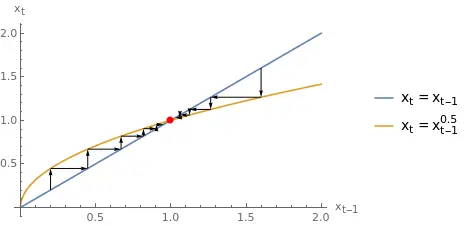
Starting from $x_{0} < \bar{x}_{2}$, the variable slowly increases until it reaches the steady state $\bar{x}_{2}.$ Notice how the curvature of the function decreases (and is smaller than one), generating the convergence. We can reason similarly for the case $x_{0} > \bar{x}_{2}.$

First-order systems of difference equations

A system of first-order difference equations takes the form:

$$\begin{eqnarray} x^{1}_{t+1} & = f^{1}(x^{1}_{t}, \ldots, x^{N}_{t}), \\\ \vdots & \\\ x^{N}_{t+1} & = f^{N}(x^{1}_{t}, \ldots, x^{N}_{t}). \end{eqnarray}$$

As before, we often interested by the steady states of first-order systems of difference equations. Finding a steady state implies solving the system for a fixed point $(\bar{x}^{1}, \ldots, \bar{x}^{N})$ such that

$$\begin{eqnarray} \bar{x}^{1} & = f^{1}( \bar{x}^{1}, \ldots, \bar{x}^{N}), \\\ \vdots & \\\ \bar{x}^{N} & = f^{N}( \bar{x}^{1}, \ldots, \bar{x}^{N}). \end{eqnarray}$$

Example: suppose the following system of first-order difference equations:

$$\begin{eqnarray} x_{t} & = 0.3x_{t-1} + y_{t-1}^{0.5}, \\\ y_{t} & = x_{t-1} - 0.5y_{t-1}. \end{eqnarray}$$

Finding the steady states requires solving the system of equations:

$$\begin{eqnarray} \bar{x} & = 0.3 \bar{x} + \bar{y}^{0.5}, \\\ \bar{y} & = \bar{x} - 0.5 \bar{y}. \end{eqnarray}$$

The system has two solutions: $(\bar{x}_{1}, \bar{y}_{1}) = (0,0)$ and $(\bar{x}_{2}, \bar{y}_{2}) = (1.36, 0.90).$

Stability of a first-order system of difference equations

Let the functions $f^{1}(\cdot), \ldots, f^{N}(\cdot)$ be differentiable and let $(\bar{x}^{1}, \ldots, \bar{x}^{N})$ be a steady state of the dynamic system. Moreover, assume the steady state is interior on the domain $\mathcal{J}\in \mathbb{R}^{N}.$ The steady state is locally stable if for any initial value $(x^{1}_{0}, \ldots, x^{N}_{0})$ near enough to $(\bar{x}^{1}, \ldots, \bar{x}^{N})$ the dynamics of $(x^{1}_{0}, \ldots, x^{N}_{0})$ converge to $(\bar{x}^{1}, \ldots, \bar{x}^{N}).$

It may be difficult to assess whether the previous condition applies. Note: de la Croix and Michel provide a more technical version on pages 320–321. Instead, we can analyse the stability of the system using a first-order Taylor approximation around the steady state and applying a technique similar to what we used for the single-equation case.

First, a first-order Taylor approximation of $f^{1}$ around the steady state is given by

$$f^{1}(x^{1}, \ldots, x^{N}) - f^{1}(\bar{x}^{1}, \ldots, \bar{x}^{N}) \simeq \sum_{i=1}^{N} {f^{1}_{i}}^{\prime}(\bar{x}^{1}, \ldots, \bar{x}^{N})(x^{i} - \bar{x}^{i}),$$

and similarly for $f^{2}(\cdot), \ldots, f^{N}(\cdot).$ We can express these in matrix notation:

$$ \begin{pmatrix} x^{1}_{t+1} - x^{1}_{t} \\\ \vdots \\\ x^{N}_{t+1} - x^{N}_{t} \end{pmatrix} = \bar{A} \begin{pmatrix} x^{1}_{t} - \bar{x}^{1} \\\ \vdots \\\ x^{N}_{t} - \bar{x}^{N} \end{pmatrix}, $$ where $\bar{A}$ is an $N \times N$ matrix of the derivatives of $f^{1}(\cdot), \ldots, f^{N}(\cdot)$ taken at the point $(\bar{x}^{1}, \ldots, \bar{x}^{N})^{\prime},$ called Jacobian matrix:

$$\bar{A} = \begin{pmatrix} {f^{1}_{x_{1}}}^{\prime}(\bar{x}^{1}, \ldots, \bar{x}^{N}) & \ldots & {f^{1}_{x_{N}}}^{\prime}(\bar{x}^{1}, \ldots, \bar{x}^{N}) \\\ \vdots & \vdots & \vdots \\\ {f^{N}_{x_{1}}}^{\prime}(\bar{x}^{1}, \ldots, \bar{x}^{N}) & \ldots & {f^{N}_{x_{N}}}^{\prime}(\bar{x}^{1}, \ldots, \bar{x}^{N}) \end{pmatrix} $$

Note: the matrix $\bar{A}$ is evaluated at the steady state $(\bar{x}^{1}, \ldots, \bar{x}^{N})$.

Hyperbolicity of the hyperplane

Assume that functions $f^{1}(\cdot), \ldots, f^{N}(\cdot)$ are continuously differentiable in $\mathcal{J}$. Let $(\bar{x}^{1}, \ldots, \bar{x}^{N})$ be a steady state in $\mathcal{J}.$ If the moduli of the eigenvalues of the Jacobian are different from 1 $(|\lambda_{1}| \neq 1, \ldots, |\lambda_{N} \neq 1),$ then the steady state is hyperbolic. If any of the eigenvalues equals 1, then the steady state is non-hyperbolic.

However, even if the steady state is non-hyperbolic, adequately choosing the initial conditions for the control variables can put it in a saddle-path trajectory, this is, one that leads to the steady state. In that case, we need some eigenvalues to be within the unit circle: $(-1,1).$

A steady state is stable if all the eigenvalues associated to the Jacobian matrix are inside the unit circle $(-1,1).$ This is, if we denote the eigenvalues by $\lambda_1, \lambda_2,\ldots, \lambda_N,$ the steady state is stable if and only if $\lambda_i \in (-1,1), i=1,\ldots,N.$

In many economic applications we often find that one eigenvalue is outside the unit circle. Blanchard-Kahn characterises the types of steady states.

One important type is the saddle path. In such case, there is only one initial configuration of variables such that the economy converges towards the steady state. Any other initial set of values delivers a non-converging trajectory. In economics, we often encounter a $2 \times 2$ system. Often, the initial value of one variable is fixed (state variable, in general capital). Hence, we have to select the value of the other variable (control variable, in general consumption) in such a way that it is on the saddle path.

We develop a full example in Example.