The phase diagram

Note: based on Section 2.3 of Romer, Advanced Macroeconomics.

The Ramsey model is fully described by two dynamic equations:

$$\left. \begin{eqnarray} u^{\prime}(c_{t}) = \beta(f^{\prime}(k_{t+1}) + 1 - \delta)u^{\prime}(c_{t+1}), \\\ k_{t+1} = f(k_{t} + (1-\delta)k_{t} - c_{t}. \end{eqnarray} \right\} \tag{8.1, Equilibrium} \label{eq:eq} $$

The phase diagram is a representation on the $(c,k)$ plane of all the stationary points for $c$ and $k.$ This is, we plot all $(c,k)$ combinations such that $c$ is constant, and all the $(c,k)$ combinations such that $k$ is constant. The set of points $(c,k)$ implying a constant consumption is called the $c$-locus. Similarly, we have the $k$-locus.

These loci are curves on the $(c,k)$ plane, and any intersection between them is a steady state because both $c$ and $k$ are simultaneously constant. The phase diagram is a useful tool to analyse the behaviour of a dynamic system because it indicates the direction of movement of the variables at any point on the plane.

The dynamics of $c$

The first equation of \ref{eq:eq} describes the dynamics of consumption.

$$u^{\prime}(c_{t}) = \beta ( f^{\prime}(k_{t+1}) + 1 - \delta) u^{\prime}(c_{t+1}).$$

Rearranging it we arrive at:

$$\frac{u^{\prime}(c_{t})}{u^{\prime}(c_{t+1})} = \beta ( f^{\prime}(k_{t+1}) + 1 - \delta).$$

In the phase diagram we want to plot combinations of $(c,k)$ such that $c$ is constant. Constant consumption implies $c_t = c_{t+1} \implies \frac{u^\prime (c_t)}{u^\prime (c_{t+1})} = 1.$ Therefore, the $c$-locus is

$$ 1 = \beta ( f^{\prime}(k_{t+1}) + 1 - \delta)$$

and any level of capital satisfying it implies constant consumption. This condition depends only on the level of capital.

Denote such level $k^{\star}$.
When $k < k^{\star}, f^{\prime}(k) > f^{\prime}(k^{\star})$, implying that $u^{\prime}(c_{t}) > u^{\prime}(c_{t+1})$ and hence consumption will raise over time. Similarly, if $k > k^{\star}$ implies that consumption falls. Note: remember that we are looking at $f^{\prime}(k)$ and $u^{\prime}(c)$, not $k$ and $c.$ This information is summarised in the following Figure.

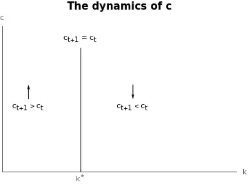
The arrows show the direction in which consumption $c$ evolves. As discussed before, consumption raises when capital is below $k^{\star}$ and raises when above. Note the vertical line: it denotes the level of capital $k^{\star}$ such that $c$ is constant. The value $k^{\star}$ can be easily computed: $k^{\star} = {f^{\prime}}^{-1}\left(\frac{1-\beta (1-\delta)}{\beta}\right).$

The dynamics of $k$

We can proceed similarly with the motion of capital. The relevant equation in this case is:

$$k_{t+1} = f(k_{t}) + (1- \delta)k_{t} - c_{t}.$$

As before, we are interested in the combinations of $(k,c)$ such that capital remains constant over time. In this case, though, and contrasting with the previous, we will obtain that both capital and consumption affect capital levels in the future: production uses current capital, and current consumption depletes current production. We can rearrange the previous equation to obtain the following:

$$k_{t+1} - k_{t} = f(k_{t}) - \delta k_{t} - c_{t}.$$ Setting $k_{t+1} = k_{t} \implies k_{t+1} - k_{t} = 0$ so capital is constant yields:

$$ 0 = f(k_{t}) - \delta k_{t} - c_{t} \implies c_{t} = f(k_{t}) - \delta k_{t}.$$

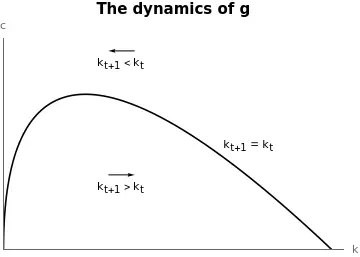
In the $(k,c)$ space, the equation takes a form similar to a parabola: it combines production —with decreasing marginal returns— with a linear depreciation rate. In fact, $f(k_t)-\delta k_t$ admits one maximum $(f^\prime (k_t) = \delta)$ the Golden rule we discuss later. Since $f^{\prime \prime}(k_t)<0,$ the stationary point is a maximum.

Let’s now analyse how capital evolves when consumption is above and below the level that makes it constant. From $k_{t+1} - k_{t} = f(k_{t}) - \delta k_{t} - c_{t}$, if consumption is above the level we have that $k_{t+1} - k_{t} < 0,$ meaning that capital decreases over time. The opposite applies when consumption is below the level that guarantees a constant level of capital. The Figure below summarises these findings:

The phase diagram

We can combine the information above to produce the phase diagram. It indicates the motion of variables at different points of the $(k,c)$ space.

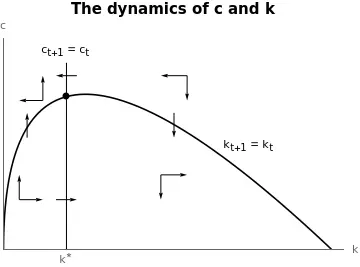
The arrows show the motion of each variable at different combinations of $(k,c).$ For instance, to the left of the $c$-locus and above the $k0$-locus consumption increases and capital decreases. Finally, the point indicating the intersection of both curves is the steady state: all variables remain constant at their values.