Introduction

Ricardo’s model of international trade is based on the idea of comparative advantage and predicts that countries gain from trade because they have different productivities. Yet, the reason for productivity differentials comes from different technology: $z_x,z_y$ are different from $z_x^\star,z_y^\star$ (actually, what matters is $\frac{z_x}{z_y} \neq \frac{z_x^\star}{z_y^\star}$).

However, countries also have different endowements so that, even if they have the same technology, they may have different productivities because they will use the inputs in different proportions.

For example, a country endowed with plenty of capital and little labor has a comparative advantage in goods that require lots of capital, but little labor — such as grains. If capital abounds, its price is low. Also, because capital is the main production factor in capital intesive industries, the price of capital-intensive goods will be low. Labor-intensive goods, on the other hand, are very expensive to produce since labor is scarce and its price is high. Therefore, the country is better off importing those goods.

Therefore, according to the Hecskcher-Ohlin model, the comparative advantage is due to the fact that nations have various factors of production with varying endowments.

Factor intensities, and an example

Factor intensity measures the relationship between capital and labor in the production of a good. This is, the capital intensity is the ratio:

\begin{equation} \frac{K}{L} \end{equation}

We will see later how to compute it. A key element of the Heckscher-Ohlin model is that one sector is capital intensive while the other is labor intensive. An important remark is that, in the model, the capital intensive industry is capital intensive for each level of production. This is, there are no reversals.

Suppose we have an industry producing one good with capital and labor. We assume that this good is capital intensive, which means that the capital-labor ratio used in this industry is large. Let $Y = K^{0.8}L^{0.2}$ be the production function of this good. We can compute, for instance, how much does it cost to produce 100 units of this good. \begin{align} \min_{L,K}, & w L + r K \\ \text{s.t.}, & Y = K^{0.8}L^{0.2} = 100 \end{align}

The minimum cost (difficult to solve) is: $125 \times 4^\frac{1}{5} w^\frac{1}{5} r^\frac{4}{5}$. Suppose we had prices $w=a$ and $r=b$ with $a>b$ because labor is scarce. The cost of producing is $125 \times 4^\frac{1}{5} a^\frac{1}{5} b^\frac{4}{5}$. Would the cost decrease if the the prices were reversed, $w=b$ and $r=a$? The answer is no: \begin{align} 125 \times 4^\frac{1}{5} b^\frac{1}{5} a^{4/5} &< 125 \times 4^\frac{1}{5} a^\frac{1}{5} b^{4/5} \\ b^\frac{1}{5} a^{4/5} & < a^\frac{1}{5} b^{4/5} \\ a^\frac{3}{5} & < b^\frac{3}{5} \\ a < b \end{align} Which is a contradiction because we assumed $a > b$.

This hints to the general idea that, because the industry is capital intensive, it benefits from having aboundant capital.

2 Goods, 2 Factors, 2 Countries

Despite the model focusing on trade, which necessitates two countries, we begin the analysis with one country only to understand how production decisions are made.

As stated before, we will consider that production functions (this is, technology) are the same across countries. However, each sector has a specific production function involving two factors of production: capital and labor. The total labor force in the country is $L$ and the total amount of capital is $K$. The economy produces two goods, as before: xboxes and yogurt.

Because each sector uses capital and labor for production, let $L_x$ and $L_y$ be the amount of labor used in the production of xboxes and yogurt, respectively. Similarlly, let $K_x$ and $K_y$ be the amount of capital used in the production of xboxes and yogurt, respectively. Mirroring the Ricardian model, production factors are perfectly mobile across sectors, but not across countries.

The production functions are: \begin{align} Q_x &= \mathcal{X}(K_x, L_x) \\ Q_y &= \mathcal{Y}(K_y, L_y) \end{align}

Some standard assumptions apply to $\mathcal{X}$ and $\mathcal{Y}$:

• Production is increasing in both factors of production.
  • $\frac{\partial \mathcal{X}}{\partial j_x} > 0, j \in {K, L}$
  • $\frac{\partial \mathcal{Y}}{\partial j_y} > 0, j \in {K, L}$
• The marginal product of each factor is decreasing in the amount of that factor used.
  • $\frac{\partial^2 \mathcal{X}}{\partial j_x^2} < 0, j \in {K, L}$
  • $\frac{\partial^2 \mathcal{Y}}{\partial j_y^2} < 0, j \in {K, L}$
• The production functions are homogenous of degree one
  • $\mathcal{X}(tK_x, tL_x) = t\mathcal{X}(K_x, L_x)$
  • $\mathcal{Y}(tK_y, tL_y) = t\mathcal{Y}(K_y, L_y)$
  • More on that on Homogenous Functions.

Consumers have preferences (as in Ricardo) over the consumption of both goods. Moreover, preferences are also the same in both countries, so this cannot drive trade. With preferences being represented by \begin{align} U(Q_x, Q_y) \end{align} we impose utility to be increasing in both arguments:

• $\frac{\partial U}{\partial Q_j} > 0, j \in {x, y}$

Autarky

In autarky, consumption equals production because there is no trade. Let’s find out how the country determines the amout of xboxes and yogurt to produce.

Production and Factor Allocation

First, production. The country has a total amount of capital $K$ and a total amount of labor $L$, and we assume perfect competition. A representative firm in the xbox sector maximizes profits: \begin{align} \max_{K_x, L_x} \pi_x &= P_x Q_x - w_x L_x - r_x K_x \\ \text{s.t.} & Q_x = \mathcal{X}(K_x, L_x) \end{align}

The maximization problem can be solved using by substituting $Q_x = \mathcal{X}(K_x, L_x)$ into the objective function and maximizing with respect to $K_x$ and $L_x$. \begin{align} \frac{\partial \mathcal{L}}{\partial K_x} &= P_x \frac{\partial \mathcal{X}}{\partial K_x} - r_x = 0 \\ \frac{\partial \mathcal{L}}{\partial L_x} &= P_x \frac{\partial \mathcal{X}}{\partial L_x} - w_x = 0 \\ \\ p_x \frac{d \mathcal{X}}{d K_x} &= r_x \\ p_x \frac{d \mathcal{X}}{d L_x} &= w_x \end{align}

If we compute the wage-rental ratio for the xbox sector, we get an optimality condition: \begin{align} \frac{w}{r} &= \frac{\mathcal{X}_L}{\mathcal{X}_K} = \frac{MPL_x}{MPK_x} \end{align}

Where the term $MPL_x$ is the marginal product of labor in the xbox sector and $MPK_x$ is the marginal product of capital in the xbox sector and the ratio $\frac{MPL_x}{MPK_x}$ is called the marginal rate of technical substitution. The marginal rate of technical substitution is the rate at which the country can substitute capital for labor in the xbox sector so that the level of output remains constant. We can easily check this by differentiating the production function: $0 = \mathcal{X}_K \mathrm{d}K_x + \mathcal{X}_L \mathrm{d}L_x \implies \frac{\mathcal{d}K_x}{\mathcal{d}L_x} = -\frac{\mathcal{X}_L}{\mathcal{X}_K} = -\frac{MPL_x}{MPK_x}$

To see why it represents optimality, suppose $\frac{w_x}{r_x} < \frac{MPL_x}{MPK_x}$. If we use one less unit of capital (K) and substitute it with labor (L) according to the MRTS, we can maintain the same level of output. The cost saving from using one less unit of labor is $w_x$. If we decrease labor by one unit, we must increase capital by $\frac{MPL_x}{MPK_x}$ units. This costs $r_x \frac{MPL_x}{MPK_x}$. Since $w_x < r_x \frac{MPL_x}{MPK_x}$, we can save more by substituting capital with labor. So any situtation where $\frac{w_x}{r_x} \neq \frac{MPL_x}{MPK_x}$ is not optimal.

Graphically, when $\frac{w_x}{r_x}$ increases, the labor to capital ratio decreases. Intuitively, when $\frac{w_x}{r_x}$ increases, hiring workers becomes more expensive relative to hiring capital. Consequently, firms will hire less labor and more capital. By decreasing the number of workers $MPL_x$ increases, and by having more capital $MPK_x$ decreases. Therefore, $\frac{MPL_x}{MPK_x}$ increases, too. But $\frac{L}{K}$ rises!

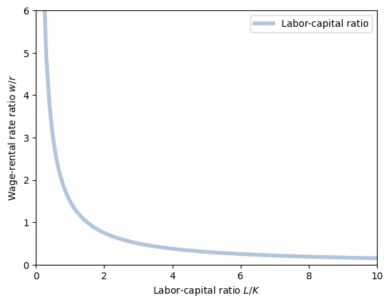
Example

Suppose a Cobb-Douglas production function for xboxes such as \begin{equation} \mathcal{X} = K_x^\xi L_x^{1-\xi},\quad \xi \in (0,1) \end{equation} $\xi$ is the Greek letter xi, for xbox.

The marginal products of labor and capital are: \begin{align} \mathcal{X}_L &= (1-\xi) K_x^\xi L_x^{-\xi} \\ \mathcal{X}_K &= \xi K_x^{\xi-1} L_x^{1-\xi} \end{align}

Hence, profit maximization implies: \begin{align} \frac{w_x}{r_x} &= \frac{\mathcal{X}_L}{\mathcal{X}_K} = \frac{(1-\xi) K_x^\xi L_x^{-\xi}}{\xi K_x^{\xi-1} L_x^{1-\xi}} = \frac{1-\xi}{\xi} \frac{K_x}{L_x} \end{align}

As we showed before, when $\frac{w_x}{r_x}$ increases, the labor to capital ratio decreases. This is because $\frac{w_x}{r_x}$ increases, hiring workers becomes more expensive relative to hiring capital.

Because we have two sectors, we can write the same equation for the yogurt sector: \begin{align} w_y &= p_y \frac{\partial \mathcal{Y}}{\partial L_y} \\ r_y &= p_y \frac{\partial \mathcal{Y}}{\partial K_y} \\ \\ \frac{w_y}{r_y} &= \frac{\mathcal{Y}_L}{\mathcal{Y}_K} = \frac{MPL_y}{MPK_y} \end{align}

Now, workers and capital can move freely between the two sectors. If the wage in the xbox sector were higher than the wage in the yogurt sector, workers would move from the yogurt sector to the xbox sector. Consequently, no yogurt would be produced. In general, this is sub-optimal because typically one imposes the Inada conditions in the utility function. The Inada conditions indicate that marginal utilities are infinite when consumption of a good is zero, so that utility can be massively increased by moving from zero to some positive consumption. Since in autarky consumption must be equal to production, this means that if consumers want to always consume some good, production of that good must be positive. In general, to be able to produce something both production factors must be present, meaning that wages must be the same in both sectors so that workers work in both.

Using the same reasoning, we conclude that rental rates must be equal in both sectors because capital can move freely between the two sectors. Hence $w_x = w_y = w$ and $r_x = r_y = r$.

This implies that $\frac{w_x}{r_x} = \frac{w_y}{r_y}$ and therefore the marginal rates of technical substitution are equal in both sectors. \begin{align} \frac{w_x}{r_x} &= \frac{w_y}{r_y} \implies \\ \frac{MPL_x}{MPK_x} &= \frac{MPL_y}{MPK_y} \end{align}

As we will see in more detail when talking about the Standard Trade Model, this condition already implies that we can write labor in one sector as a function of capital in that same sector (or write capital as a function of labor). Moving from here to a PPF is a simple step, but often mathematically involved and impossible to solve analytically.

Factor intensity

Let’s go back to our example where $\mathcal{X} = K_x^\xi L_x^{1-\xi}$, which lead to $\frac{w_x}{r_x} = \frac{1-\xi}{\xi} \frac{K_x}{L_x}$. Assume that yogurts also have a Cobb-Douglas production function, but exponent, $\mathcal{Y} = K_y^\upsilon L_y^{1-\upsilon}$, where $\upsilon$ is the Greek letter “upsilon”.

In the yogurt sector, we will have \begin{align} \frac{w_y}{r_y} &= \frac{1-\upsilon}{\upsilon} \frac{K_y}{L_y} \end{align}

Since $\frac{w_x}{r_x} = \frac{w_y}{r_y}$, we thus have \begin{align} \frac{1-\xi}{\xi} \frac{K_x}{L_x} &= \frac{1-\upsilon}{\upsilon} \frac{K_y}{L_y} \implies \end{align}

Let’s suppose that $\xi > \upsilon$, meaning the capital is more producive in the xbox sector than in the yogurt sector. How does it affect the ratio of capital to labor?

\begin{align} \frac{1-\xi}{\xi} \frac{K_x}{L_x} &= \frac{1-\upsilon}{\upsilon} \frac{K_y}{L_y} \implies \\ \frac{\frac{K_x}{L_x}}{\frac{K_y}{L_y}} &= \frac{1-\upsilon}{\upsilon} \frac{\xi}{1-\xi} \\ \end{align}

Because $\xi > \upsilon$, the right-hand side is larger than one.

This implies that capital intensity is higher in the xbox sector than in the yogurt sector. This is $\frac{K_x}{L_x} > \frac{K_y}{L_y}$. Note that, in the plot, we have $\frac{L}{K}$. Because the yogurt sector is more labor intense, its curve lies to the right of the xbox sector.

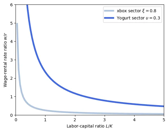
Finally, we know that the total amount of labor and capital must be divided between the two industries. \begin{align} L_x + L_y &= L \\ K_x + K_y &= K \end{align}

This means that the conutry-wide labor-capital ratio is: \begin{align} \frac{L}{K} &= \frac{L_x + L_y}{K} \\ &= \frac{L_x}{K_x} \frac{K_x}{K} + \frac{L_y}{K_y} \frac{K_y}{K} \\ \end{align} This expression indicates that, at the country level, the capital-labor ratio is a weighted average of the capital-labor ratios in the two sectors. The weights are the shares of capital in each sector. Here the term $\frac{L}{K}$ is the relative supply of labour, while the term $\frac{L_x}{K_x} \frac{K_x}{K} + \frac{L_y}{K_y} \frac{K_y}{K}$ is the relative demand. Note that, supply is given and fixed.

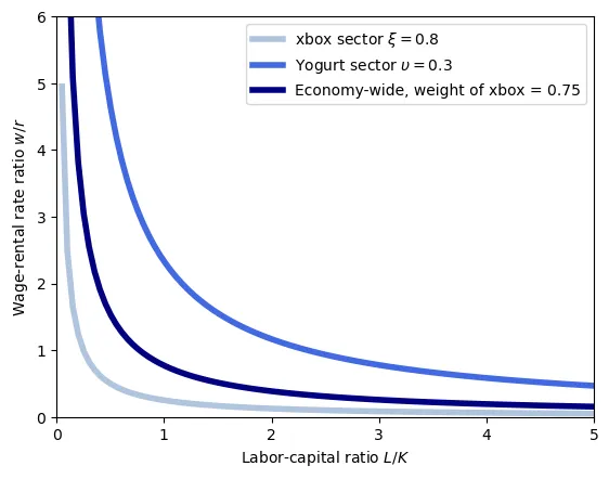
Therefore, given the relative wage-to-rental-rate ratio, the capital-labor ratio in each sector, and the total amount of labor and capital, we can determine the country-wide capital-labor ratio.

The Stolper-Samuelson Theorem

The Stolper-Samuelson theorem studies the effect of a change in the relative price of a good on the relative remuneration of the two factors of production and the real remuneration of each factor.

The theorem states that:

• If the relative price of the good produced by the labor-intensive sector increases, then the relative wage increases ($\frac{w}{r} \uparrow$), the real wage increases and the real rental rate decreases.
• Or, alternatively, if the relative price of the good produced by the capital-intensive sector increases, then the relative wage decreases ($\frac{w}{r} \downarrow$), the real wage decreases and the real rental rate increases.

This is, the Stolper-Samuelson Theorem indicates that, when prices change, there are winners and losers. Therefore, when a country opens up to trade, we know that the good it exports will increase in price, and the good it imports will decrease in price. Consequently, and differently from the Ricardian model, under Hecksher-Ohlin, opposition to trade from the importing sector is (partily) rational. Nevertheless, the gains from trade as suffficiently large to outweigh the losses, allowing the winners to fully compensate the losers and still be better off. Hence, trade remains Pareto-improving.

Let’s prove the Stolepr-Samuelson theorem. First, let’s go back to the first-order conditions in both sectors: \begin{align} w_x &= p_x PML_x \\ w_y &= p_y PML_y \\ r_x &= p_x PMP_x \\ r_y &= p_y PMP_y \end{align} and recalling that to have production in both sectors we must have $w_x = w_y$ and $r_x = r_y$, then we can also re-arrange the expressions to get: \begin{align} w &= p_x MPL_x = p_y MPL_y \implies \frac{p_x}{p_y} = \frac{MPL_y}{MPL_x} \\ r &= p_x MPK_x = p_y MPK_y \implies \frac{p_x}{p_y} = \frac{MPK_y}{MPK_x} \end{align}

Now, we are in a good position to analyze what happens when $\frac{p_x}{p_y}$ changes. Assume that $\frac{p_x}{p_y}$ increases, so xboxes become more expensive relative to yogurt. Then, because $\frac{p_x}{p_y} = \frac{MPL_y}{MPL_x}$, it must be that $\frac{MPL_y}{MPL_x}$ increases. If $MPL_y$ increases, this indicates that $L_y$ has decreased. Alternatively, it can also be the case that $PML_x$ decreases, meaning that $L_x$ has increased. So, the first thing we notice is that, when the price of xboxes increases, labor moves from the yogurt sector to the xbox sector.

Using the second equation we can see the effects on capital. Indeed, when $\frac{p_x}{p_y}$ increases, then $\frac{MPK_y}{MPK_x}$ increases. As before, this can be due to $MPK_y$ increasing, which means that $K_y$ has decreased, or $MPK_x$ decreasing, which means that $K_x$ has increased.

Overall, it is clear that when the price of xboxes increases, capital and labor move from the yogurt sector to the xbox sector. Therefore, the production of xboxes increases and the production of yogurt decreases.

How does this affect the wage-to-rental-rate ratio? We know that the economy-wide labor-capital ratio follows: \begin{align} \frac{L}{K} &= \frac{L_x}{K_x} \frac{K_x}{K} + \frac{L_y}{K_y}\frac{K_y}{K} \end{align}

When $\frac{p_x}{p_y}$ increases, capital moves to the xbox sector ($K_x \uparrow$) which increases the weight of the xbox sector in the labor demand. Moreover, xbox production is capital-intensive, meaning that for any wage-to-rental-rate ratio, $\frac{L_x}{K_x} < \frac{L_y}{K_y}$. Then, the economy-wide labor-capital ratio $\frac{L}{K}$ becomes closer to the xbox sector’s labor-capital ratio $\frac{L_x}{K_x}$. As a consequence, $\frac{w}{r}$ falls for all levels $\frac{L}{K}$.

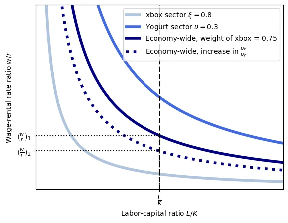
Intuitively, when $\frac{p_x}{p_y}$ increases, firms want to produce more xboxes because they are more profitable. To do so, capital and labor in the xbox industry must increase. Now, let’s suppose we move one unit of capital from the yogurt sector to the xbox sector. Because the capital intensity in the xbox sector is higher than in the yogurt sector ($\frac{K_x}{L_x} > \frac{K_y}{L_y}$), for each unit of capital in the xbox sector, we need less workers than those that will be freed in the yogurt sector. So, workers are in excess supply and the wage rate must adjust downwards to clear the market.

Lastly, at the new equilibrium, both sectors deepened their labor-capital intensity, this is, the ratio $\frac{L}{K}$ increases, as indicated by the graph (and because $\frac{w}{r}$ is inversely related to $\frac{L}{K}$ in all sectors).

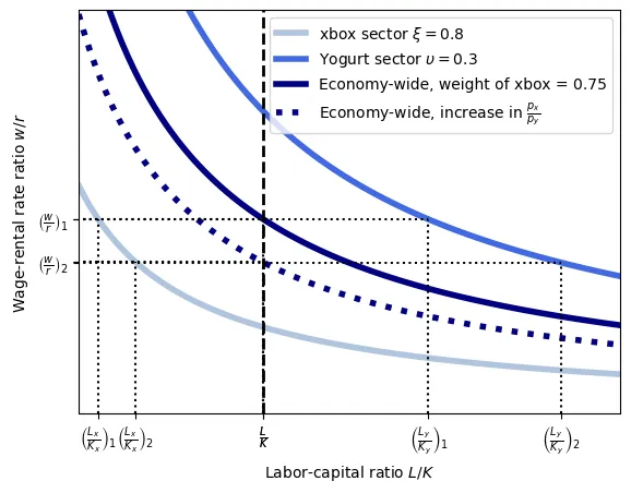
For instance, if $\frac{K_x}{L_x} = 2 \implies K_x = 2 L_x$ and $\frac{K_y}{L_y} = 1 \implies K_y = 1 L_y$, then moving 10 units of capital from the yogurt sector to the xbox sector requires adding 5 workers to the xbox sector. Yet, because we moved 10 units of capital from the yogurt sector, we have to decrease employment by 10 workers in the yogurt sector. So, we have an excess of 5 workers that will push the wage down.

Finally, we can study who wins and who looses from an increase in $\frac{p_x}{p_y}$. We do so by analyzing the real wage and the real capital return, this is, $\frac{w}{p_x}$, $\frac{w}{p_y}$ and $\frac{r}{p_x}$, $\frac{r}{p_y}$.

Production factors are paid their marginal productivity: \begin{align} r &= p_x MPK_x \quad \text{and} \quad r = p_y MPK_y \\ \frac{r}{p_x} &= MPK_x \quad \text{and} \quad \frac{r}{p_y} = MPK_y \end{align}

We also had: \begin{align} \frac{w}{r} &= \frac{MPL_x}{MPK_x} \\ \frac{w}{r} &= \frac{MPL_y}{MPK_y} \end{align}

Because $\frac{w}{r}$ decreases, the marginal product of labor must decrease and the marginal product of capital increases. Importantly, this happens in both sectors.

The real wage expressed in terms of xboxes is $\frac{w}{p_x}$. From the first-order conditions $w = p_x MPL_x$ we thus have $\frac{w}{p_x} = MPL_x$. Since $MPL_x$ decreases, the real wage decreases. The same is true if we express the real wage in terms of yogurts. From the first-order condition $w = p_y MPL_y$ we have $\frac{w}{p_y} = MPL_y$. Since $MPL_y$ decreases, the real wage decreases.

By the same token, we can see that real capital return increases in both sectors. Starting from the first order conditions $r = p_x MPK_x$ and $r = p_y MPK_y$, we have $\frac{r}{p_x} = MPK_x$ and $\frac{r}{p_y} = MPK_y$. So, the real capital return increases when we express it in terms of xboxes or yogurts.

Example

Suppose that $\mathcal{X} = K_x^\frac{2}{3} L_x^\frac{1}{3}$ and $\mathcal{Y} = K_y^\frac{1}{3} L_y^\frac{2}{3}$. From the optimality conditions (and equality of wages and returns) we have: \begin{align} \frac{w}{r} &= \frac{\frac{1}{3} K_x^\frac{2}{3} L_x^\frac{-2}{3}}{\frac{2}{3} K_x^\frac{-1}{3} L_x^\frac{1}{3}} = \frac{1}{2} \frac{K_x}{L_x} \\ \frac{w}{r} &= \frac{\frac{2}{3} K_y^\frac{1}{3} L_y^\frac{-1}{3}}{\frac{1}{3} K_y^\frac{-2}{3} L_y^\frac{2}{3}} = 2 \frac{K_y}{L_y} \\ \end{align} From here, we can derive the labour-capital ratios as functions of $\frac{w}{r}$: \begin{align} \frac{L_x}{K_x} &= \frac{1}{2} \left(\frac{w}{r}\right)^{-1} \\ \frac{L_y}{K_y} &= 2 \left(\frac{w}{r}\right)^{-1} \\ \end{align}

Hence, in equilibrium we must have: \begin{equation} \frac{L}{K} = \frac{L_x}{K_x} \frac{K_x}{K} + \frac{L_y}{K_y}\frac{K_y}{K} \end{equation}

Substituting the labour-capital ratios from above, we get: \begin{align} \frac{L}{K} &= \frac{1}{2} \left(\frac{w}{r}\right)^{-1} \frac{K_x}{K} + 2 \left(\frac{w}{r}\right)^{-1} \frac{K_y}{K} \implies \\ \frac{w}{r} &= \frac{K}{L}\left(\frac{1}{2}\frac{K_x}{K} + 2\frac{K_y}{K}\right) \end{align} Finally, because $K = K_x + K_y$ \begin{equation} \frac{w}{r} = \frac{K}{L}\left(\frac{1}{2}\frac{K_x}{K} + 2\frac{(K-K_x)}{K}\right) \end{equation} Therefore, when $K_x$ increases, $\frac{w}{r}$ decreases because $\frac{\partial \frac{w}{r}}{\partial K_x} = \frac{K}{L}\left(\frac{1}{2}\frac{1}{K} - 2\frac{1}{K}\right) = -\frac{K}{L}\frac{1}{2} < 0$.

We also have the following relationship: \begin{align} \frac{p_x}{p_y} &= \frac{\frac{2}{3}K_y^\frac{1}{3} L_y^\frac{-1}{3}}{\frac{1}{3}K_x^\frac{2}{3}L_x^\frac{-2}{3}} = 2 \frac{K_y^\frac{1}{3} L_x^\frac{2}{3}}{K_x^\frac{2}{3} L_y^\frac{1}{3}} \\ \frac{p_x}{p_y} &= \frac{\frac{1}{3}K_y^\frac{-2}{3}L_y^\frac{2}{3}}{\frac{2}{3}K_x^\frac{-1}{3}L_x^\frac{1}{3}} = \frac{1}{2}\frac{K_x^\frac{1}{3}L_y^\frac{2}{3}}{K_y^\frac{2}{3}L_x^\frac{1}{3}} \\ \end{align}

Again, because $K = K_x + K_y$, and $L = L_x + L_y$, we can write: \begin{align} \frac{p_x}{p_y} &= 2 \frac{(K-K_x)^\frac{1}{3} L_x^\frac{2}{3}}{K_x^\frac{2}{3} (L - L_x)^\frac{1}{3}} \\ \frac{p_x}{p_y} &= \frac{1}{2}\frac{K_x^\frac{1}{3}(L-L_x)^\frac{2}{3}}{(K-K_x)^\frac{2}{3}L_x^\frac{1}{3}} \end{align}

Suppose that $\frac{p_x}{p_y} = 0.75$ and that $L = 10 , K = 20$. Then:

\begin{align} 0.75 &= 2 \frac{(20-K_x)^\frac{1}{3} L_x^\frac{2}{3}}{K_x^\frac{2}{3} (10 - L_x)^\frac{1}{3}} \\ 0.75 &= \frac{1}{2}\frac{K_x^\frac{1}{3}(10-L_y)^\frac{2}{3}}{(20-K_x)^\frac{2}{3}L_x^\frac{1}{3}} \\ \\ \\ K_x &= 10.8642, L_x = 2.2917, K_y = 9.1358, L_y = 7.7083 \end{align}

Then, from, \begin{equation} \frac{w}{r} = \frac{K}{L}\left(\frac{1}{2}\frac{K_x}{K} + 2\frac{(K-K_x)}{K}\right) \end{equation} we can retrieve the wage-rental ratio $\frac{w}{r} = 2.37$ The real wage in terms of $x$ is $\frac{w}{p_x} = MPL_x = 0.94$, in terms of $y$ is 0.70 and the real rental rate is $\frac{r}{p_x} = 0.39$ and $\frac{r}{p_y} = 0.2976$

If $\frac{p_x}{p_y}$ increases to $0.8$, then: \begin{align} 0.8 &= 2 \frac{(20-K_x)^\frac{1}{3} L_x^\frac{2}{3}}{K_x^\frac{2}{3} (10 - L_x)^\frac{1}{3}} \\ 0.8 &= \frac{1}{2}\frac{K_x^\frac{1}{3}(10-L_y)^\frac{2}{3}}{(20-K_x)^\frac{2}{3}L_x^\frac{1}{3}} \\ \\ \\ K_x &= 13.6458, L_x = 3.493, K_y = 6.3541, L_y = 6.506 \end{align}

And the wage-rental ratio decreases to $\frac{w}{r} = 1.9531$ The real wage in terms of $x$ is $\frac{w}{p_x} = MPL_x = 0.826$, in terms of $y$ is 0.661 and the real rental rate is $\frac{r}{p_x} = 0.423$ and $\frac{r}{p_y} = 0.3386$

Consequently, as predicted, when the relative price of the capital-intensive good increases, the wage-rental ratio decreases, the real wage decreases, and the real rental rate increases.

The Rybczynski Theorem

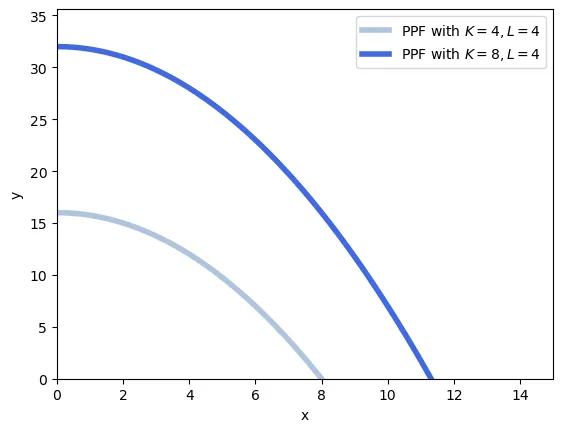
The Rybczynski theorem states that at constant relative goods prices, a rise in the endowment of one factor will lead to a more than proportional expansion of the output in the sector which uses that factor intensively, and an absolute decline of the output of the other good. This is, in general, an increase in a country’s endowment of a factor will cause an increase in output of the good which uses that factor intensively, and a decrease in the output of the other good.

Let’s suppose that our country experiences a population increase. According to the theorem, the yogurt sector (intensive in labor) will increase its production more than proportionally, and the xbox sector (intensive in capital) will decrease its production.

We can easily verify this. From \begin{equation} \frac{L}{K} = \frac{L_x}{K_x} \frac{K_x}{K} + \frac{L_y}{K_y}\frac{K_y}{K} \end{equation} an increase in $L$ means that the left-hand side increases in value. Because yogurts are labor-intensive $\left(\frac{K_x}{L_x} > \frac{K_y}{L_y} \implies \frac{L_y}{K_y} > \frac{L_x}{K_x} \right)$, to increase the right-hand side of the equation we need to increase $\frac{K_y}{K}$, and thus decrease $\frac{K_x}{K}$. Moving capital to the yogurt sector increases its production.

The Hecksher-Ohlin Theorem

Let’s suppose now that we finally have two countries: Home and Foreign. Each country is endowed with labor $L, L^\star$ and capital $K, k^\star$. There are two sectors in each country: xbox and yogurt. Production technology is the same in both countries, this is, $x = \mathcal{X}(K, L)$ and $y = \mathcal{Y}(K, L)$. Consumers also have the same preferences over xboxes and yogurts in both countries indicated by $u(x,y)$.

The Hecksher-Ohlin theorem states that in the long run, the country that is relatively more abundant in a factor will specialize in the production of the good that uses that factor intensively. Let’s derive it!

To begin with, we suppose that Home and Foreign have exactly the same endowments. $L = L^\star$ and $K = K^\star$. Becuase they also have the same technology and preferences, trade does not occur. Their internal prices are identical, and thus the international price will also coincide with the two autarky prices. The relative supply of labor with respect to capital at the world level is: \begin{equation} \frac{L + L^\star}{K + K^\star} \end{equation}

Now, let’s shift some capital from Foreign to Home, such that Home is capital abundant and Foreign labor abundant. \begin{equation} \frac{L}{K} < \frac{L + L^\star}{K + K^\star} < \frac{L^\star}{K^\star} \end{equation}

The Rybczynski theorem tells us that Home will increase its production of xboxes and decrease its production of yogurts, because xboxes are capital-intensive. With exactly the same preferences, Home will have an excess supply of xboxes (alternatively, the price of xboxes at Home will be lower than in Foreign), so it will export xboxes and import yogurts.

The implication is clear:

• When a country opens up to international trade, it will specialize in the production of the good that uses the factor that it is relatively more abundant in.

Moreover, from the Stolper-Samuelson theorem we also know that capital owners will benefit from trade in Home, and workers will benefit from trade in Foreign.

Solving the model

We need to find the allocations $K_x, L_x, K_y, L_y, x, y, w, r, K_x^\star, L_x^\star, K_y^\star, L_y^\star, x^\star, y^\star, \frac{p_x}{p_y}$ given endowments $K, L, K^\star, L^\star$, production functions and preferences.

First, from the maximization of profits, we can derive: \begin{align} w &= p_x \frac{\partial \mathcal{X}(K_x,L_x)}{\partial L_x} = p_y \frac{\partial \mathcal{Y}(K_y,L_y)}{\partial L_y} \\ r = p_x \frac{\partial \mathcal{X}(K_x,L_x)}{\partial K_x} &= p_y \frac{\partial \mathcal{Y}(K_y,L_y)}{\partial K_y} \\ \\ w^\star &= p_x \frac{\partial \mathcal{X}(K_x^\star,L_x^\star)}{\partial L_x^\star} = p_y \frac{\partial \mathcal{Y}(K_y^\star,L_y^\star)}{\partial L_y^\star} \\ r^\star = p_x \frac{\partial \mathcal{X}(K_x^\star,L_x^\star)}{\partial K_x^\star} &= p_y \frac{\partial \mathcal{Y}(K_y^\star,L_y^\star)}{\partial K_y^\star} \end{align}

From the maximization of utility, we get the labor-capital ratio in each sector as a function of prices by solving: \begin{align} \frac{MPL_x}{MPK_x} &= \frac{MPL_y}{MPK_y} \\ \frac{MPL_x^\star}{MPK_x^\star} &= \frac{MPL_y^\star}{MPK_y^\star} \end{align}

Once we have $\frac{L}{K}$ as a function of prices we can get the wage-to-rental rate also as a function of prices. It is important to note that wages and rental rates depend only on labor-capital ratios and the prices, not on the endowment. At this stage, we have \begin{align} \frac{L_x}{K_x} &= f\left(\frac{p_x}{p_y}\right) \\ \frac{L_y}{K_y} &= g\left(\frac{p_x}{p_y}\right) \\ \frac{L_x^\star}{K_x^\star} &= f^\star\left(\frac{p_x}{p_y}\right) \\ \frac{L_y^\star}{K_y^\star} &= g^\star\left(\frac{p_x}{p_y}\right) \\ \frac{w}{r} = h\left(\frac{p_x}{p_y}\right) \\ \frac{w^\star}{r^\star} = h^\star\left(\frac{p_x}{p_y}\right) \end{align}

From here, we can use $\frac{L}{K} = \frac{L_x}{K_x} \frac{K_x}{K} + \frac{L_y}{K_y} \frac{K_y}{K}$ to get the allocations in each sector as a function of prices. Because $\frac{L}{K}$ is given (the country endowment) we can solve: \begin{align} \frac{L}{K} &= f\left(\frac{p_x}{p_y}\right) \frac{K_x}{K} + g\left(\frac{p_x}{p_y}\right) \frac{K-K_x}{K} \end{align}

And thus, retrieve $K_x$ and $K_y = K - K_x$ as a function of prices. Finally, we can use $K_x$ and $L_x$ to find the amount produced in the xbox sector as a function of prices, and the same applies to yogurts. This can of course done for both countries.

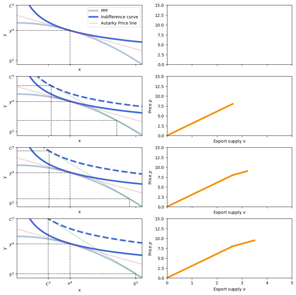
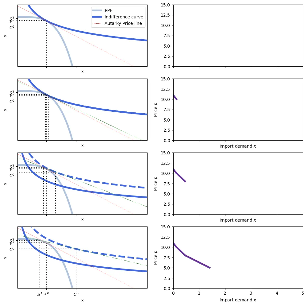
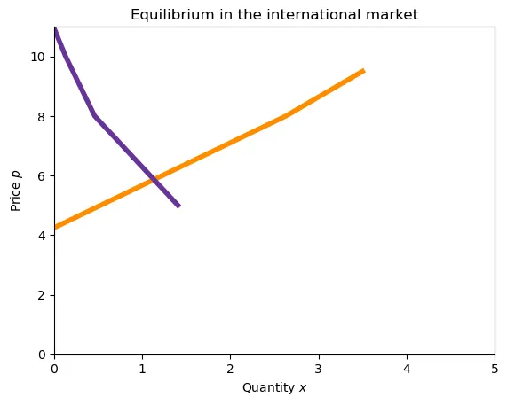
To obtain the equilibrium price level with trade, we use the utility function to derive the demand for each good as a function of prices. This is quite involved (specially if non-homothetic function are used) but the idea is to get the demand for each good as a function of prices. From it, we can compute the supply of exports of xboxes from one country and the demand o imports of xboxes from the other country. Equating supply of exports to demand of imports yields the equilibrium price.

Example

Let $\mathcal{X} = K_x^\frac{1}{2} L_x^\frac{1}{2}$ and $\mathcal{Y} = K_y^\frac{1}{3} L_y^\frac{2}{3}$. Hence, the xbox sector is capital intensive while the yogurt sector is labor intensive.

Let’s solve for the model. First, we need to find the labor-capital ratio in each sector as a function of prices. Maximizing profits at home: \begin{align} max_{K_x,L_x} &\ \pi = p_x \mathcal{X} - w L_x - r K_x \\ 0 &= \frac{\partial \pi}{\partial K_x} \implies r = p_x \frac{1}{2} K_x^{-\frac{1}{2}} L_x^\frac{1}{2} \\ 0 &= \frac{\partial \pi}{\partial L_x} \implies w = p_x \frac{1}{2} K_x^\frac{1}{2} L_x^{-\frac{1}{2}} \\ \max_{K_y,L_y} &\ \pi^\star = p_y \mathcal{Y} - w^\star L_y - r^\star K_y \\ 0 &= \frac{\partial \pi^\star}{\partial K_y} \implies r = p_y \frac{1}{3} K_y^{-\frac{2}{3}} L_y^\frac{2}{3} \\ 0 &= \frac{\partial \pi^\star}{\partial L_y} \implies w = p_y \frac{2}{3} K_y^\frac{1}{3} L_y^{-\frac{1}{3}} \end{align}

Because $w$ and $r$ are the same in both sectors: \begin{align} p_x \frac{1}{2} K_x^{-\frac{1}{2}} L_x^\frac{1}{2} &= p_y \frac{1}{3} K_y^{-\frac{2}{3}} L_y^\frac{2}{3} \\ p_x \frac{1}{2} K_x^\frac{1}{2} L_x^{-\frac{1}{2}} &= p_y \frac{2}{3} K_y^\frac{1}{3} L_y^{-\frac{1}{3}} \\ \\ \frac{p_x}{p_y} &= \frac{\frac{1}{3} K_y^{-\frac{2}{3}} L_y^\frac{2}{3}}{\frac{1}{2} K_x^{-\frac{1}{2}} L_x^\frac{1}{2}} = \frac{2}{3}\frac{K_x^\frac{1}{2}L_y^\frac{2}{3}}{K_y^\frac{2}{3}L_x^\frac{1}{2}} = \frac{2}{3} \left(\frac{L_x}{K_x}\right)^\frac{-1}{2} \left(\frac{L_y}{K_y}\right)^\frac{2}{3} \\ \frac{p_x}{p_y} &= \frac{\frac{2}{3} K_y^\frac{1}{3} L_y^{-\frac{1}{3}}}{\frac{1}{2} K_x^\frac{1}{2} L_x^{-\frac{1}{2}}} = \frac{4}{3} \frac{K_y^\frac{1}{3}L_x^\frac{1}{2}}{K_x^\frac{1}{2}L_y^\frac{1}{3}} = \frac{4}{3} \left(\frac{L_x}{K_x}\right)^\frac{1}{2} \left(\frac{L_y}{K_y}\right)^\frac{-1}{3} \end{align}

From the second we can write: \begin{equation} \left(\frac{L_x}{K_x}\right)^\frac{1}{2} = \frac{3}{4} \frac{p_x}{p_y} \left(\frac{L_y}{K_y}\right)^\frac{1}{3} \end{equation}

Re-arranging the first equation gives: \begin{equation} \left(\frac{L_x}{K_x}\right)^\frac{1}{2} = \frac{2}{3} \left(\frac{p_x}{p_y}\right)^{-1} \left(\frac{L_y}{K_y}\right)^\frac{2}{3} \end{equation}

Thus, replacing: \begin{align} \frac{3}{4} \frac{p_x}{p_y} \left(\frac{L_y}{K_y}\right)^\frac{1}{3} &= \frac{2}{3} \left(\frac{p_x}{p_y}\right)^{-1} \left(\frac{L_y}{K_y}\right)^\frac{2}{3} \\ \frac{9}{8} \left(\frac{p_x}{p_y}\right)^2 &= \left(\frac{L_y}{K_y}\right)^\frac{1}{3} \\ \frac{L_y}{K_y} &= \left(\frac{9}{8}\right)^3 \left(\frac{p_x}{p_y}\right)^6 \end{align}

We have found the labor-capital ratio in the yogurt industry as a function of prices. Then, we can use $ \left(\frac{L_x}{K_x}\right)^\frac{1}{2} = \frac{3}{4} \frac{p_x}{p_y} \left(\frac{L_y}{K_y}\right)^\frac{1}{3} \implies \frac{L_x}{K_x} = \left(\frac{3}{4}\right)^2 \left(\frac{p_x}{p_y}\right)^{2} \left(\frac{L_y}{K_y}\right)^\frac{2}{3}$ to retrieve $\frac{L_x}{K_x}$: \begin{equation} \frac{L_x}{K_x} = \left(\frac{3}{4}\right)^2 \left(\frac{p_x}{p_y}\right)^{2} \left(\frac{9}{8}\right)^2 \left(\frac{p_x}{p_y}\right)^4 = \left(\frac{27}{32}\right) ^2\left(\frac{p_x}{p_y}\right)^6 \end{equation}

The next step is to find use the country endowments to derive $K_x$, $L_x$ and $K_y$, $L_y$ as a function of prices. \begin{align} \frac{L}{K} &= \frac{L_x}{K_x}\frac{K_x}{K} + \frac{L_y}{K_y}\frac{K_y}{K} \\ \frac{L}{K} &= \left(\frac{27}{32}\right)^2 \left(\frac{p_x}{p_y}\right)^6 \frac{K_x}{K} + \left(\frac{9}{8}\right)^3 \left(\frac{p_x}{p_y}\right)^6 \frac{K-K_x}{K} \\ K_x &= \frac{2\left(729 K \left(\frac{p_x}{p_y}\right)^6 - 512 L\right)}{729 \left(\frac{p_x}{p_y}\right)^6} = 2K - \frac{1024}{729}L \left(\frac{p_x}{p_y}\right)^{-6} \end{align} Therefore, we also have $K_y = K - K_x = \frac{1024}{729}L\left(\frac{p_x}{p_y}\right)^{-6}-K$.

We can corroborate already that, when $\frac{p_x}{p_y}$ increases, $K_x$ increases and $K_y$ decreases. Next, let’s find the levels $L_x$ and $L_y$: \begin{align} \frac{L_y}{K_y} &= \left(\frac{9}{8}\right)^3 \left(\frac{p_x}{p_y}\right)^6 \implies L_y = 2L - \frac{729}{512}K \left(\frac{p_x}{p_y}\right)^6 \\ \frac{L_x}{K_x} &= \left(\frac{27}{32}\right)^2 \left(\frac{p_x}{p_y}\right)^6 \implies L_x = \frac{729}{512}K \left(\frac{p_x}{p_y}\right)^6 - L \end{align} Here we can also confirm that when $\frac{p_x}{p_y}$ increases, $L_x$ increases and $L_y$ decreases. So, when $\frac{p_x}{p_y}$ increases, the production of $x$ increases and the production of $y$ decreases.

We can indeed find the production as a function of prices: \begin{align} x = \mathcal{X}(K_x,L_x) = \left(2K - \frac{1024}{729}L \left(\frac{p_x}{p_y}\right)^{-6}\right)^\frac{1}{2} \left(\frac{729}{512}K \left(\frac{p_x}{p_y}\right)^6 - L\right)^\frac{1}{2} \\ y = \mathcal{Y}(K_y,L_y) = \left(\frac{1024}{729}L\left(\frac{p_x}{p_y}\right)^{-6}-K\right)^\frac{1}{3} \left(2L - \frac{729}{512}K \left(\frac{p_x}{p_y}\right)^6\right)^\frac{2}{3} \end{align}

This closes the supply part of the Hecksher-Ohlin model. The next step is to derive the demand for $x$ and $y$ as a function of prices so that we can compute exports and imports. We use here a simple utility formulation: $u(x,y) = \log(x) + \log(y)$.

With the country producing the previously derived quantities, this means that utility has to be maximized on an isovalue line passing through that point and with slope equal to the relative prices. This is: \begin{align} \max_{x,y} &= \log(x) + \log(y) \\ \text{s.t.} & p_x x + p_y y = \\ &= p_x \left(2K - \frac{1024}{729}L \left(\frac{p_x}{p_y}\right)^{-6}\right)^\frac{1}{2} \left(\frac{729}{512}K \left(\frac{p_x}{p_y}\right)^6 - L\right)^\frac{1}{2} + \\ &+ p_y \left(\frac{1024}{729}L\left(\frac{p_x}{p_y}\right)^{-6}-K\right)^\frac{1}{3} \left(2L - \frac{729}{512}K \left(\frac{p_x}{p_y}\right)^6\right)^\frac{2}{3} \end{align}

From here, the maths become very messy (even more than what we have now)! Once we maximize, we can obtain the demand for $x$ as a function of prices. From here, determining the supply of exports is simple: production ($\mathcal{X}$) minus consumption. Because we have the same production and utility function for both countries, demand for imports will be consumption minus production. Note that we wrote the function without replacing values for $K$ and $L$, which will differ between countries and give rise to trade. Finally, equating yields the equilibrium price level.

Factor prize equalization

Without trade, capital earns less at Home than in Foreign because Home is capital-abundant, and labor earns more because Home is labor-abundant. Similarly, the relative price of xboxes will be lower in Home before trade.

When coutries open up to trade, the price of goods converges and becomes unique. This price convergence also implies that factors earn the same in both countries: trade equalizes factor prices. Indeed, as we saw before, wages and rents do not depend on the endowment of each country.

From the set of conditions: \begin{align} \frac{p_x}{p_y} &= \frac{MPK_y}{MPK_x} = \frac{MPL_y}{MPL_x} \\ \frac{p_x}{p_y} &= \frac{MPK_y^\star}{MPK_x^\star} = \frac{MPL_y^\star}{MPL_x^\star} \\ \end{align}

We can find that equal labor-capital ratios must prevail for each sector across countries. This is: \begin{align} \left(\frac{L_x}{K_x}\right) &= \left(\frac{L_x}{K_x}\right)^\star \\ \left(\frac{L_y}{K_y}\right) &= \left(\frac{L_y}{K_y}\right)^\star \\ \end{align}

Then, because $\frac{w}{r} = \frac{MPL_x}{MPK_x} = \frac{MPL_y}{MPK_y}$, and $\frac{w^\star}{r^\star} = \frac{MPL_x^\star}{MPK_x^\star} = \frac{MPL_y^\star}{MPK_y^\star}$, we have that $\frac{w}{r} = \frac{w^\star}{r^\star}$. This is, the relative factor costs are the same across countries. Finally, it is possible to show that the price of each factor is also the same between countries: $w = w^\star$ and $r=r^\star.$ This is, factor prices equalize.

In essence, when two countries trade, they are effectively trading factors of production. If Home is labor abundant, for instance, it lets Foreign use some of its workers, not by selling labor but by exporting goods that were produced with a high labor-to-capital ratio. Indeed, the goods that Home sells use much more labour that what it receives, so more labor is embodied in Home’s exports.