The Standard Trade Model

Introduction

The previous models seen in the first half of the course focus on particular aspects that may give rise to international trade. In particular, the Ricardian model emphasizes differences in comparative advantages that can be ultimately related to different production functions. The Heckscher-Ohlin model places the emphasis on the relative abundance of production factors.¹ However, when dealing with real-world applications, these models may be too restrictive. In fact, it is quite likely that the reasons behind trade include, up to some point, all the elements that these different models highlight.

In any case, the two (three) models have some common elements, which make the building blocks of the Standard Trade Model.

• The productive capacity of an economy is determined by its production possibility frontier. Differences in this frontier give rise to trade.
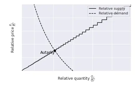
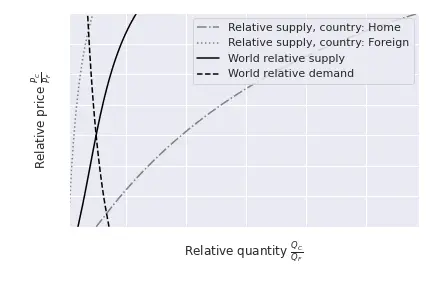
• Production possibilities (and demand) determine a country’s relative supply schedule.
• World equilibrium is determined by world relative demand and world relative supply.

The Standard Model of Trade is built of four key relationships:

1. The relationship between the production possibility frontier and the relative supply curve,
2. The relationship between relative prices and relative demand,
3. The determination of world equilibrium by world relative supply and world relative demand, and
4. The effects of the terms of trade (price of a country’s exports divided by the price of its imports) on a nation’s welfare.

Production possibility frontier and the relative supply curve

We present a situation very similar to that of the Heckscher-Ohlin model. Suppose there are only two countries in the world, Home (H) and Foreign (F), and that two products are produced in each country, Food (F) and Clothing (C). Of course, each sector is equipped with a unique technology, and in principle, technologies can be different in different countries. Underlying these production functions, we have production factors. For instance, in the Heckscher-Ohlin model we had two production factors: Capital (K) and Labour (L).

Drawing the production possibility frontier (PPF)

The possibility frontier is a function that relates the quantities produced in each sector when the production processes use the same finite resources. This is, in our case, the PPF indicates how many units of Food the economy can produce considering that it is currently producing $C$ units of clothing. Of course, we assume that production is efficient, this is, the production factors $K$ and $L$ are allocated efficiently between sectors. Note: an implicit assumption is that the economy makes use of all resources.

Consider the following production functions: $$Q_F = H(K_F, L_F), \mathrm{and}, Q_C = G(K_C,L_C).$$ Since the economy uses all the available resources, we also have that $$K = K_F + K_C, \mathrm{and}, L = L_F + L_C.$$

This process is a bit convoluted if we use generic functions. However, we first describe the general process and then go through the details using an example. The general objective is to find the maximum amount of good $F$ that the economy can produce considering that it is already producing $C$ units of clothing. Moreover, we shall assume that production of $C$ is efficient. If we then vary the amount of $C$, we can retrieve the PPF. Hence, we are really solving the following constrained maximisation problem for a given level $C = \bar{C}.$

$$\begin{align} \max_{K_F,L_F} & \, H(K_F, L_F) \\\ \mathrm{s.t.} & \, G(K_C, L_C) = \bar{C},\\\ &K=K_F + K_C, \\\ &L = L_F + L_C. \end{align}$$

If we solve for the associated Lagrangian, we obtain the condition:

$$\frac{H_{K_F}}{H_{L_F}} = \frac{G_{K_C}}{G_{L_C}}.$$ And since $K=K_F + K_C$ and $L = L_F + L_C$ $$\frac{H_{K-K_C}}{H_{L-L_C}} = \frac{G_{K_C}}{G_{L_C}}.$$

The previous expression defines a relationship between capital used in the production of clothes $K_C$ and labour used in the production of clothes $L_C.$ For suitable cases, it is possible to isolate one of the two and obtain a closed-form solution $L_C = Z(K_C),$ where $Z(\cdot)$ is a function. Lastly, we can write a parametric function for clothing and food production: $$(Q_C\,,Q_F) = (G(K_C, Z(K_C)),\, H(K-K_C, L-Z(K_C))).$$ Finally, in some particular cases we can transform the parametric equation into an explicit relationship between $C$ and $F$.

Example: Suppose that $H(K_F, L_F) = K_F^{\frac{1}{3}}L_F^{\frac{2}{3}}$ and $G(K_C,L_C) = K_C^{\frac{1}{2}} L_C^{\frac{1}{2}}.$ Since both sectors optimize, we have that $MRS$ across sectors coincide, this is, $\frac{H_{K_F}}{H_{L_F}} = \frac{G_{K_C}}{G_{L_C}}.$ In our case, we have:

$$\frac{\frac{1}{3}K_F^{-\frac{2}{3}}L_F^{\frac{2}{3}}}{\frac{2}{3}K_F^{\frac{1}{3}}L_F^{-\frac{1}{3}}} = \frac{\frac{1}{2}K_C^{-\frac{1}{2}}L_C^{\frac{1}{2}}}{\frac{1}{2}K_C^{\frac{1}{2}}L_C^{-\frac{1}{2}}}.$$ Or, after some simplifications, $$\frac{1}{2}\frac{L_F}{K_F} = \frac{L_C}{K_C} \implies 2 L_C K_F = L_F K_C.$$ Since $K=K_F + K_C$ and $L = L_F + L_C$, we have, $$2 L_C (K - K_C) = (L - L_C) K_C \implies L_C = \frac{L K_C}{2K - K_C}.$$ Finally, we can substitute everything in the production functions to obtain the parametric functions:

$$\begin{align} (Q_C,\, Q_F) &= \left(G(K_C, L_C),\, H(K_F, L_F)\right) = \\\ &=\left(G\left(K_C, \frac{L K_C}{2K - K_C}\right),\, H\left(K-K_F, L-\frac{L K_C}{2K - K_C}\right)\right) = \\\ &=\left(K_C^\frac{1}{2} \left(\frac{L K_C}{2K - K_C}\right)^\frac{1}{2},\, (K-K_C)^\frac{1}{3} \left(L-\frac{L K_C}{2K - K_C}\right)^\frac{2}{3}\right). \end{align}.$$

Last, we can isolate $K_C$ from the equation for $C$ and obtain $$K_C = \frac{Q_C \sqrt{Q_C^2+8LK}-Q_C^2}{2L}.$$ Finally, we can plug this expression for $K_C$ into the parametric equation of $F$ and obtain the quantity of food that the economy can produce as a function of the number of clothing: $$\begin{align} & Q_F = \\\ & = \left(K-\frac{Q_C \sqrt{Q_C^2+8LK}-Q_C^2}{2L}\right)^\frac{1}{3} \left(L-\frac{L\frac{Q_C \sqrt{Q_C^2+8LK}-Q_C^2}{2L}}{2K -\frac{Q_C \sqrt{Q_C^2+8LK}-Q_C^2}{2L}}\right)^\frac{2}{3} \end{align}$$ If we assume, for a second, that the economy counts with $10$ units of labour $(L=10)$ and $5$ units of capital $(K=5)$, then the production possibility frontier has the following shape:

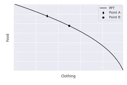
Deciding how much to produce

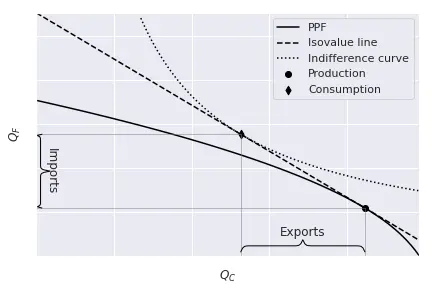
The PPF only indicates all the possible combinations of clothing and food that the economy can produce. For instance, points such as $A$ and $B$ are feasible, so is any other point on the PPF. The point at which the economy produces depends on the relative price of cloth relative to food: $\frac{P_C}{P_F}.$ In particular, for prices $P_C$ and $P_F$, the economy will maximise the value of its total production, this is, the economy maximises $$V = Q_C P_C + Q_F P_F.$$ Levels $V$ are called isovalue lines: combinations of $Q_C$ and $Q_F$ that produce the same value $V.$

Considering, for instance, that $P_C = 7$ and $P_F = 6$, we can draw several isolines corresponding to different values $V$. The next figure draws isovalue lines for values $V = {20,40,60}.$

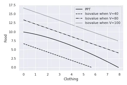
To draw one isovalue line for a given $V$, we isolate the variable in the vertical axis, this is, $Q_F$ in our case: $$V = Q_C P_C + Q_F P_F \implies Q_F = \frac{V}{P_F} - \frac{P_C}{P_F}Q_C.$$ As is clear, as we increase the $V$, the isovalue lines move away from the origin. Also, the slope of all the isovalue lines is the same (unless we change prices) and it corresponds to the relative price of $Q_C,$ $-\frac{P_C}{P_F}.$ So, for a given set of prices $P_C$ and $P_F$, the economy chooses the combination $(Q_C^\star, Q_F^\star)$ that maximises the value $V.$ This is, the economy solves the following problem:

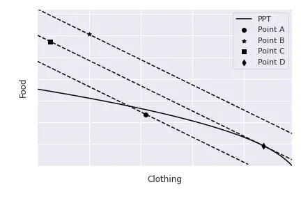
$$\begin{align} \max_{Q_C, Q_F} & P_C Q_C + P_F Q_F \\\ \mathrm{s.t.} & \, Q_F = F(Q_C) \end{align},$$ where $Q_F = F(Q_C)$ represents the PPF, because the amount of food the economy is produces depends on the number of cloth it produces, as we have just seen. If we solve this maximisation we obtain the following optimality condition: $$F^\prime(Q_C) = -\frac{P_C}{P_F}.$$ This condition indicates that the economy will produce at the point in which the PPF is tangent to the isovalue line. This is normal: suppose that we selected a point such as $A$ below. At this point, the economy is not producing at its full capacity because it is inside the PPF. We already know that we can increase the value of total production if we move the isovalue line away from the origin. Points like $B$ or $C$ are not feasible, because they are above the PPF and, thus, the economy cannot produce these combinations $Q_C$ and $Q_F$ with its available resources $K$ and $L$. Thus, it is optimal to lie on the point that is the farthest away which still touches the PPF: the tangency point $D$.

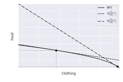
When the relative price changes, the slope of the isovalue lines change. For instance, if $P_C$ increases, making clothing more valuable, the slope (in absolute value) increases. This has the consequence of changing the optimal point. In particular, if $P_C$ increases, the economy can become richer by shifting production to clothing, because its price increases. Graphically, the new point of tangency is characterised by an increase in $Q_C$ and, consequently, a decrease in $Q_F.$ Mathematically, we can see this because we know that $Q_F$ is a function of $Q_C$, for instance, $Q_F = F(Q_C).$ Therefore, the optimal production point is characterised by, as we just saw, $$F^\prime(Q_C) = -\frac{P_C}{P_F}.$$ If we compute the how $Q_C$ changes with a change in $P_C$ we obtain:

$$\frac{\partial Q_C}{\partial P_C} = - \frac{1}{P_F F^{\prime \prime}(Q_C)}.$$ Looking at the form of $F(Q_C)$, we know that $F^{\prime \prime}(Q_C)$ is negative ($F^{\prime \prime}(Q_C)$), and therefore, $$\frac{\partial Q_C}{\partial P_C} = - \frac{1}{P_F F^{\prime \prime}(Q_C)} > 0.$$ So, as the intuition suggested, when the price of clothing increases, the economy produces more of it. We could also show that the quantity of food decreases. Hence, the relative supply of cloth $\left(\frac{Q_C}{Q_F}\right)$ increases. Finally, we can draw the relative supply curve of the economy, this is, how $\left(\frac{Q_C}{Q_F}\right)$ changes when the relative price $\left(\frac{P_C}{P_F}\right)$ changes. As $Q_C$ increases and $Q_F$ decreases following the rise if $P_C$, it is easy to see that the ration $\frac{Q_C}{Q_F}$ will increase as well.

Individuals’ preferences and the relative demand curve

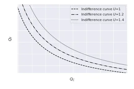
The tastes of an individual are represented by a series of indifference curves: the set of points on the $(Q_C, Q_F)$ plane that generate a utility level $\bar{U}.$ These indifferences curves have three main properties:

• Are downward sloping: if an individual receives less units of food, she has to be compensated with more clothing to achieve the same utility level.
• Curves farther away from the origin represent higher levels of welfare, this is, higher values $\bar{U}.$
• For a given curve, it becomes flatter as one moves to the right.

Mathematically, we can write the indifference curves by plotting $\bar{U} = U(Q_C, Q_F)$ for different values of $\bar{U}$, where $U(\cdot, \cdot)$ represents the utility function. The next Figure plots several indifference curves, with values $\bar{U} = {1, 1.2, 1.4}$ and using $U(Q_C, Q_F) = \log(Q_C)+\log(Q_F).$

Considering that the economy can trade at the prices $P_C,\, P_F$, individuals will optimize according to them. Hence, they will choose a consumption bundle such that utility is maximal and tangent to the relative price line.² Note: without trade, the efficient point will be one such that the PPF and the indifference curves are tangent, which would determine the prices within the country. Hence, given prices $P_C$ and $P_F$, consumers maximize:

$$\begin{align} &\max_{Q_C,\, Q_F} U(Q_C,\, Q_F) \\\ & \mathrm{s.t.}\, P_C Q_C + Q_F P_F = V \end{align}$$

where $V$ represents the total value of production. Such equilibrium is represented in the Figure below:

As we did before, we can consider the effect of an increase in $\frac{P_C}{P_F}$. First, as we already knew, the economy produces more clothing $C$ and less food $F$. This is because the relative price of clothing with respect to food increased, and it is more profitable to produce and sell clothing. Hence, the value of total production has increased (the economy produces more of the good that has become more expensive). On the other side of the market, consumers’ income has also increased: the total income of an economy is the total value of production. Effectively, this means that the new equilibrium indifference curve must lie on the isovalue line. However, consumers face two effects:

• A wealth effect: now that income is larger, they want to consume more of all goods,
• A substitution effect: the rise in $P_C$ relative to $P_F$ makes consuming clothing less attractive because it costs more. Therefore, consumers tend to consume less of $C$ and more of $F$.

Depending on the utility representation, one effect dominates the other (and for the utility choice we made, one exactly cancels out the other).

Similar to the relative supply curve, we can draw a relative demand curve which represents the relative demand $\frac{Q_C}{Q_F}$ with respect to the relative price $\frac{P_Q}{P_F}.$

The terms of trade

When the relative price of clothing increases, this is, when $\frac{P_C}{P_F}$ increases, a country that exports clothing is better off. And, by the same token, when the relative price of clothing falls, that country is in a worse position. Of course, these effects depend on whether the country exports clothing or food.

To have a better way of tracking the effects of price changes, we define the terms of trade as the price of the good a country initially exports divided by the price of the good that it imports. In general, a rise in the terms of trade increases a country’s welfare, and a decline in the terms of trade reduces its welfare. However, it is important to remark that welfare can never be below its level under autarky: if that were the case, the economy would just stop trading.

Two countries

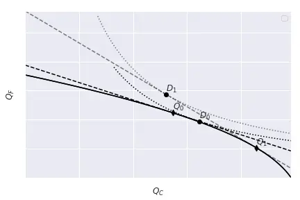
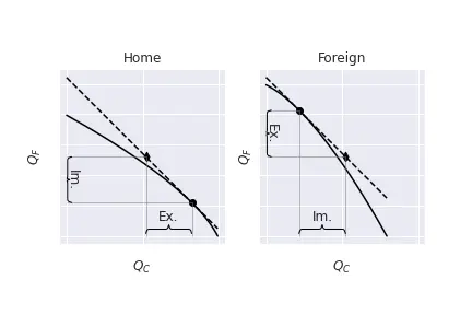
We now introduce two countries in our analysis. We assume that both countries produce the two goods, but Home exports cloth while Foreign exports food. The terms of trade of Home are measured as $\frac{P_C}{P_F}$ while Foreign’s are $\frac{P_F}{P_C}$. Lastly, we suppose that trade arises because of fundamental differences in the production technology, which will be reflected in their PPF and their relative supply curves. For instance, Home is more productive in producing cloth. To simplify, we assume that demand in both countries is exactly the same. As usual, equilibrium points are found by equalizing the slope of the PPF in each country to the world relative prices, as depicted below:

The world-level relative supply of clothing and food can be computed by aggregating from the country level: $$\frac{Q_C^{world}}{Q_F^{world}} = \frac{Q_C + Q_C^\star}{Q_F + Q_F^\star}.$$ Note that, in reality, the world relative supply is a weighted average of each country’s relative supply curve. Hence, the world relative supply always lies in between the two countries’ relative supply curves. We can proceed similarly for world relative demand. However, since we assumed that demand is exactly the same in both countries, the world relative demand will coincide be equal to the relative demand curve of either country. The Figure below illustrates the case:

Growth, the terms of trade and welfare

A classical question in international economics concerns the effects of biased economic growth on trade and, hence, welfare. If all other countries in the world grow, is it good or bad for our economy? It is possible to argue in the positive and in the negative sense:

• If other countries grow, it means that the market size for our exports increases, so we can export and sell, hence we are better off.
• But our firms also face higher competition from the foreign countries, which hurts welfare in our country. Similarly, if it is our country the one that grows, we also have opposite effects:
• If we are growing, we produce more and we can sell of this additional production abroad.
• But also, by increasing production the price of the goods falls, so we earn less from exporting, which has a negative effect on welfare.

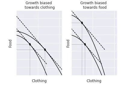
In reality, whether growth is positive or negative heavily depends on the direction of growth. First, economic growth means that we can produce more of all goods, so that PPF moves outwards. However, growth typically benefits more one sector than the others: we call this biased growth. Graphically, it means that the PPF moves outwards much more for one sector than the other. The figure below depicts and exaggerated case. What is really important is that, for unchanged relative prices, the economy produces more of the good in which there is a bias and less of the other. For instance, if there is biased growth in terms of clothing, the economy will produce more clothing and less food. We can intuitively see this by studying the optimisation problem. Before, we have established that we can write the amount of labour in each sector as a function of capital: $L_C = L(K_C).$ We also know that capital and labour not employed in the clothing industry will be used in the food industry, hence $K_F = K - K_C$ and $L_F = L - L_C = L - L(K_C).$ Thus, in fact, given the relative price, the economy only has to determine how much capital to allocate to the clothing sector, and optimality conditions will tell us how much labour we shall allocate to it. Lastly, market clearing will indicate the amounts of capital and labour in the food sector. So, the economy solves: $$\max_{K_C} p F\left(K_C, L(K_C)\right) + G\left(K - K_C, L - L(K_C)\right),$$ where $p$ represents the relative price $\frac{P_C}{P_F}.$ Taking the derivative with respect to $K_C$ $$\begin{align} &\frac{\partial p F\left(K_C, L(K_C)\right) + G\left(K - K_C, L - L(K_C)\right)}{\partial K_C} = 0 \implies \\\ &\implies p\left[F^\prime_K + F^\prime_L L^\prime\right] = G^\prime_K + G^\prime_L L^\prime. \end{align}$$

Biased technological growth implies unequal productivity growth, this is, the productivity increases much more in the clothing sector than in the food sector. Mathematically, this means that the derivatives $F^\prime$ increase much more than the $G^\prime.$ If the relative price $p$ remains constant, there is an imbalance in the equation: the left-hand side is larger than the right-hand side. To rebalance it, we shall make $F^\prime$ decrease and $G^\prime$ increase, and this happens when $K_C$ increases. So, with more capital in the clothing sector, the economy clearly produces more clothing and less food.

Of course, biased growth towards clothing implies an increase in the relative supply (of clothing), while an biased growth towards food implies a decrease in the relative supply (of clothing). So we can now answer our question: Suppose Home grows, and the growth is biased towards clothing. Hence, Home’s relative supply of clothing increases at any given set of relative prices. This also implies that the world relative supply of clothing will increase, moving towards the right. As a result of that shift, in equilibrium, the new relative price of clothing decreases. If Home exported clothing, a lower relative price of clothing worsens its terms of trade, and it improve Foreign’s terms of trade (it exports food). Remark: it does not really matter which country grows, but the direction of growth. Growth biased towards the good that Home exports always worsens Home’s terms of trade; while any growth biased in the good that Home imports improves Home’s terms of trade.

Effects of economic growth

We can now analyse the effects of economic growth on welfare.

The rest of the world grows

Suppose first that the rest of the world is growing. If the growth is export-biased, this is, growth occurs in their exporting sector, this is good for us. The reason is that it improves our terms of trade: the good we import is cheaper, and welfare at home increases.

If, instead, their growth is import-biased (in the sense that they grow in the sector Foreign imports), it worsens our terms of trade: the rest of the world is growing in the sector we export. Thus, welfare at home decreases.

Home grows

Let’s focus now on what happens we Home grows. If the growth is import-biased, then these are goods news as we are growing in the sector we imported, reducing its price and improving our terms of trade. The interesting case is what happens when growth at Home is export-biased. On the one hand, this reduces our terms of trade and decreases welfare at home. However, on the other hand, Home produces more and can export more goods, which is good. In general, the increase in exports compensates the decrease in the relative price. Only when growth is extremely biased such that the price of the good really falls, then we can have immiserising growth.

• Immiserising growth In any case, during the 1950s, there were concerns about the implications of poor nations’ economic growth. Poor countries exported mostly raw materials, and growth in these countries was expected to be specially intense in the extractive sectors. This would, of course, hurt their terms of trade because these countries would experience export-biased growth. At the same time, it was likely that developed countries could create synthetic substitutes for imported raw materials, hence these countries will be import-biased growing, improving their terms of trade and worsening those of poor economies. To some, the growth of the poor economies will be make them actually worse, this is, poor economies would be better off not growing at all, insofar as export-biased growth was harmful for them. Although the possibility can arise from a theoretical model, Bhagwati (1958) shows that it only materialises when strong export-biased growth is combined with vey steep RS and RD curves.

Exercises

Some exercises to practice.