Tariffs

Tariffs

A tariff is a tax imposed on imported goods. Therefore, if a country imported goods at the world price $p^w$, after the introduction of a tariff imported goods are more expensive because they now bear an extra tax. This tax may take two forms:

• A percentage increase $p^w(1+\tau)$, called ad-valorem,
• A unitary increase $p^w + \tau$, called specific tariff.

Both are equivalent, and one can always find the corresponding percentage increase for a given unitary rise or vice-versa.

As we shall see, the effects of a tariff are different depending on the size of the country. First, we will analyze the small-country case, this is, a country whose relative size in the international markers is small and cannot influence equilibrium prices. Related to the Standard Trade model, a country is small if the changes in its supply or demand schedule do not move the world supply or demand.¹ Then, we will analyze the same tariff but when it is applied in a large country, one that has the ability to influence world prices.

Tariffs in a small, open economy

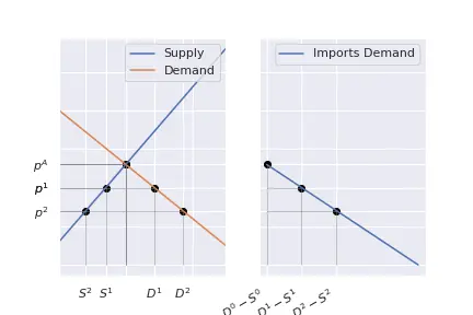
The initial situation is that of a country that is importing the good $X$. This happens because the autarkic equilibrium price, this is, the one that would prevail without trade ($p$), is higher than the world price ($p^w$) of good $X$. Then, if trade is possible and there are no tariffs, consumers will prefer to import the good and pay the lower internationa price rather than buying from the more expensive local producers. The next Figure represents this initial situation: at price $p^w$, the country experiences excess demand, hence it imports the good. Since the country is small, it can import any quantity it desires at the ongoing world price. So, the world supply curve is perfectly elastic. At price $p^w$, demand is $D^1$ and supply is $S^1$. The difference between the two is the amount of imports. As we can see, at price $p^w$ there is some local production: only the most efficient producers can supply at a price equal or lower than $p^w$. From the perspective of a local firm, the situation is simple: if it asks a price above $p^w$, sales are zero because it is always possible to import at $p^w$. If the price it asks is lower, the firm could gain more by adjusting it to $p^w$.

Next, we suppose that the government introduces a tariff $\tau > 0$ on imports. Imports are still possible, however, the price of these goods is now $p^w + \tau$. Notice that now more local firms produce: in fact, some that before were not sufficiently efficient to produce below $p^w$ can now produce because the relevant price is $p^w + \tau$. So, local supply increases. At the same time, with a higher price, demand shrinks. The combined effect is a decrease in the imports: less demand combined with a higher local supply.

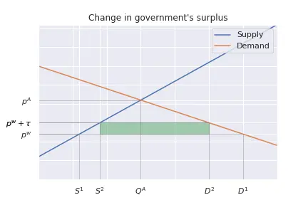
Lastly, the government raises some revenue through the tariff. For each imported good, it receives the tariff $\tau$. Therefore, the total government revenue is $(D^2 - S^2)\tau$.

Hence, after the tariff is introduced:

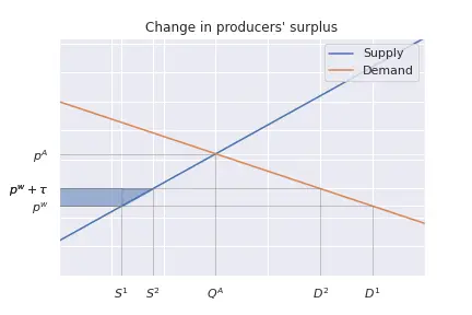
• Local producers are better off: they sell more and at a higher price.
• Consumers are worse off: the price has increased.
• The government raises some revenue. It is normal to ask: in general, is the economy better off with the tariff?

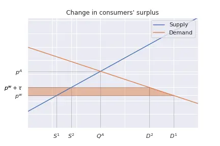
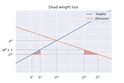
In the case of a small country the answer is no. We can proof this. Total consumer’s surplus before the tax was equal to the area below the demand curve, reaching until $D^1$, net of the purchase cost. After the tariff, their surplus only extends until $D^2$, and because $D^2 < D^1$, it is clearly smaller. However, if we aggregate all surplus changes, the entire result is a net loss of welfare, a dead-weight loss. Figures below illustrate it for linear supply and demand functions. The consumer lost surplus equal to the area represented by the orange trapezoid. The loss comprises two different aspects: consumers buy less quantity, and they do so at a higher price.

The opposite is true for producers, represented by the blue area. Notice how part of the surplus lost by consumers goes directly to the producers: they now satisfy a part of the demand that previously consisted of imports.

Lastly, the government gains the surplus depicted by the green rectangle.

If add them together, the result is that the two red triangles are lost, hence the economy as whole is worse off.

Tariffs in a large economy

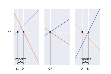
The main difference between a small and a large economy is their capacity to influence the world price. Suppose for instance that the world consists of only two countries: if Home imports the good X, then Home has monopsony power. In general, we say that a large country capable of influencing world prices faces an upwards supply curve. We can derive this curve, as well as the world demand curve, from each country’s supply and demand schedules. Suppose, for a given good, that the autarky price at Home is higher than a Foreign. Consumers at Home will be willing to import the less expensive Foreign good, and hence, there will be internation demand for imports steeming from Home. Similarly, producers in Foreign will be willing to sell goods in Home, hence, there is going to be an international supply. Next, we shall determine how much Home is willing to import. Let demand in Home $D^H(p)$, and similarly, supply will be $S^H(p)$. At the autarky price $p^H$, $D^H(p^H) = S^H(p^H).$ However, if the price was lower than that, then demand exceeds supply. 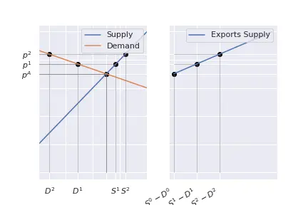The demand for imports is exactly the quantity demanded not covered with local production, this is, $$D^{W}(p) = D^H(p) - S^H(p), \forall p\leq p^H.$$ We can think similarly about international supply: $$S^{W}(p) = S^F(p) - D^F(p) \forall p\geq p^F.$$ Graphically:

Let’s suppose now that Home introduces a tariff $\tau$ for each unit imported. The world supply curve adjusts, moving up by $\tau$: if before an exporter was willing to sell at price $p$, now he will request a price $p+\tau$ to compensate for the tariff he has to pay upon entering the country.² So, for each and every quantity, the world supply curve moves up by the amount $\tau.$ A new equilibrium is formed, which solves: $$D^W(p) = S^W(p-\tau).$$ Note: the function $S^W$ indicates the quantity supplied at the price $p-\tau.$ However, in general we think of supply and demand functions as functions relating a quantity $Q$ to a price $p$, this is, $p=F(Q).$ Suppose a producer facing the tariff $\tau.$ To maintain his earnings unchanged, a producer selling $Q$ units will as a price $F(Q) + \tau$. Consequently, $p = F(Q) + \tau \implies Q=F^{-1}(p-\tau),$ and this is the reason we wrote $S^W(p-\tau)$ before.

Graphically:

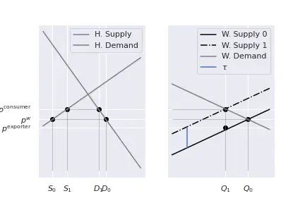
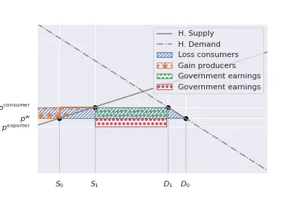
Some things must be commented:

• Althugh the tariff is $\tau$, the price payed by consumers $p^\mathrm{consumer}$ only increases by a fraction of it.
• The remaining part is absorbed by exporters, who now earn $p^\mathrm{exporter}$, which is less than before.
• As a result of the increased priced in Home:
  • Home production increases,
  • Home consumption decreases.
  • The government collects tariff duties for value $\tau (D^H(p^\mathrm{consumer}) - S^H(p^\mathrm{consumer})).$

These changes have an additional implication: A large country is able to pass a part of the dead-weight cost to the Foreign market, who now receives a smaller price for its exports. For a small country, this was a net loss for consumers. So, if a country is able to pass onto the foreign market a relatively large part of the burden imposed by a tariff, it may be better off with an import tariff than without. Graphically:

As before, the consumer’s loss (blue) is partly compensated by the producers’ increase in welfare (orange) and government revenue (green). However, a large country clearly passes away part of the losses (red), which are collected as tariffs. Then, it is possible for the red area to compensate the two blue triangles that are still lost by the consumers.

In fact, we can show that the optimal tariff is always positive As we have seen, when a country introduces a tariff of value $\tau$, a fraction of it is passed to foreign exporters and the remaining is repercuted onto the consumers. To simplify, suppose that, after the tariff $\tau$ is introduced, consumers at Home end up paying $p^w + \alpha \tau, \alpha \in (0,1)$. The total welfare in the economy is the sum of consumers’ surplus, producers’ surplus and government income raised by the tariff. Let’s denote Home supply and demand, as functions of price, by $S(p)$ and $D(p)$, respectively. Then, consumers’ surplus is given by:

$$\int_{p^w+\alpha \tau}^\infty D(p)\mathrm{d}p$$ Similarly, producers’ surplus is: $$\int_0^{p^w+\alpha \tau}S(p)\mathrm{d}p$$ And governemnt raises tariffs by value: $$\tau \underbrace{(D(p^w+\alpha \tau) - S(p^w + \alpha \tau))}_{\mathrm{Imports}}$$

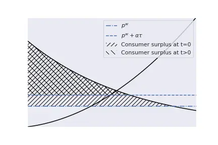
Hence, total welfare is $$\begin{align} & W(p^w, \tau) = \int_{p^w+\alpha \tau}^\infty D(p)\mathrm{d}p + \\\ & \int_0^{p^w+\alpha \tau}S(p)\mathrm{d}p + \\\ & \tau \underbrace{(D(p^w+\alpha \tau) - S(p^w + \alpha \tau))}_{\mathrm{Imports}} \end{align}$$ We study how it changes when $\tau = 0$, this is, whether, starting with no tariffs, increasing the tariff rate by a tiny amount increases or decreases welfare. To do so, we compute the derivative of total welfare with respect to $\tau$ and evaluate it at $\tau = 0$. $$\begin{align} & \left.\frac{\partial W(p^w, \tau)}{\partial \tau}\right|_{\tau = 0} = \\\ &-D(p^w+\alpha \tau) \alpha + S(p^w+\alpha \tau) \alpha + \left(D(p^w + \alpha \tau) - S(p^w+\alpha \tau)\right) = \\\ &(1-\alpha)\underbrace{\left[D(p^w+\alpha \tau) - S(p^w +\alpha \tau)\right]}_{\text{=Imports > 0}} > 0 \end{align}$$ Since the previous derivative is positive, this means that, when the tariff is zero, if we increase $\tau$ then welfare increases (as long as $\alpha \in (0,1).$ Notice also that, in the case of a small open economy, we have $\alpha = 1$, this is, the entire tariff is passed onto Home consumers. In that case, $\left.\frac{\partial W(p^w, \tau)}{\partial \tau}\right|_{\tau = 0} = 0$, meaning that a tariff $\tau = 0$ is indeed optimal. This makes sense: for a small open economy, we have seen than any positive tariff hurts the economy.

Lastly, we discuss how the value $\alpha$, this is, the part of the tariff that is passed to Home consumers, is determined. In the international market, the equilibrium price $p^w$ is determined by the intersection between the world supply and world demand. If we add a tariff, then the equilibrium price solves: $$S_w(p^w - \tau) = D_w(p^w).$$ In that case, the exporters will receive $p^w-\tau$, the consumer pays $p^w$ and $\tau$ is collected by the government. We can compute how a change in $\tau$ affects the equilibrium price: $$\begin{align} & S^\prime_w \mathrm{d}p^w - S^\prime_w \mathrm{d}\tau - D^\prime_w \mathrm{d}p = 0 \implies \\\ & \frac{\mathrm{d}p^w}{\mathrm{d}\tau} = \frac{S^\prime_w}{S^\prime_w - D^\prime_w} = \frac{\epsilon_S}{\epsilon_S-\epsilon_D} \in (0,1) \end{align}$$ where $\epsilon$ denotes the elasticity, and $\epsilon_D < 0$. Since the consumer pays $p^w$, then, the entire burden of a tariff is passed on to Home consumers when

• World supply is infinitely elastic ($\epsilon_S \rightarrow \infty$): this is the case of a small economy.
• Home demand is completely inelastic ($\epsilon_D = 0$).

Example

Suppose that we can describe the Home economy by the following supply and demand equations: $$P^{H}_{D}(q) = 10 - q, \quad P^{H}_{S}(q) = -5 + 2q.$$ We can compute the autarky equilibrium by solving $P^{H}_{S}(q) = P^{H}_{D}(q)$ which will yield the equilibrium quantity $q^{H}_{Aut.}.$ In our case, $q^{H}_{Aut.} = 5$ and the autarky price is $p^{H}_{Aut.} = 5.$ Lastly, if we assume that Home will import from the international market, we can compute the excess demand (or the demand for imports). Note: we first must find the inverse of the demand and supply, so that we can compare quantities. $$Q^{H}_{D}(p) = 10 - p, \quad Q^{H}_{S}(p) = \frac{5+p}{2}.$$ Therefore, demand for imports will be: $$Q^{I}(p) = Q^{H}_{D}(p) - Q^{H}_{S}(p) = \frac{15-3p}{2}, \quad p < 5$$

Furthermore, suppose that Foreign has the following supply and demand schedules $$P^{F}_{D}(q) = 31 - 3q, \quad P^{F}_{S}(q) = -5 + q.$$ We can compute the autarky equilibrium by solving $P^{F}_{S}(q) = P^{F}_{D}(q)$ which will yield the equilibrium quantity $q^{F}_{Aut.}.$ In our case, $q^{F}_{Aut.} = 9$ and the autarky price is $p^{H}_{Aut.} = 4.$

We can already verify that Home will import and Foreign export because the autarky price at Home is larger than in Foreign. The supply of exports from Foreign is given by (again, remember to compare quantities): $$Q^{F}_{S}(p) = \frac{31 - p}{3}, \quad Q^{H}_{S}(p) = 5+p.$$ Therefore, $$Q^{E}(p) = Q^{F}_{S}(p) - Q^{F}_{D}(p) = \frac{-16 + 4p}{3}, \quad p > 4$$

Some additional notes:

• First, notice that demand for imports decreases in $p$ and supply of exports increases with $p$.
• Second, the international equilibrium price must be between the two autarky prices.

We can compute the international equilibrium price and quantity (the quantity refers to the amount of goods internationally traded). $$Q^{E}(p) = Q^{I}(p) \implies p^{Int.} = \frac{77}{17} = 4.52 \quad Q^{I} = Q^{E} = \frac{12}{17} = 0.70.$$

Suppose that Home, a large country, imposes a specific tariff on imports of value $\tau = 0.1$. We will solve the new equilibrium using three methods:

Assume that exporters pay the tariff

First, we suppose that exporters pay the tariff. This is, we assume that for every good that crosses the border, the customs charge $0.1$ and the exporter has to pay it immediately.

To understand well how the introduction of a tariff affects the supply of exports, it is important to first realize what a supply (or demand) curve indicates. In our case, we have the following expression for the supply of exports: $$Q^{E}(p) = Q^{F}_{S}(p) - Q^{F}_{D}(p) = \frac{-16 + 4p}{3}, \quad p > 4.$$ If we compute its inverse, we get: $$P^{E}(q) = 4 + \frac{3}{4} q.$$ This equation indicates the willingness to sell, this is, the monetary amount at which a seller is willing to sell $q$ units of goods. For instance, they are ready to sell $q = 4$ units at a price of $p = 7.$ In other words, to sell these $3$ units, they must receive $7$.

Consequently, once the tariff is levied, suppliers will increase the monetary amount they ask by the value of the tariff. Following with our previous example, to sell the previous $4$ units they will ask consumers $7.1$. Of these, $0.1$ will go to the customs agent, and sellers will be left with $7$, exactly the monetary amount at which they are willing to sell $4$ units.

The same argument can be applied at each and every quantity. Therefore, in general, the price at which suppliers will be willing to sell increases by the amount of the tariff. This is, $$P^{E}(q) = 4 + \frac{3}{4} q + 0.1$$

We can rewrite the equation for the demand for imports to express the price as a function of quantities $$Q^{I}(p) = Q^{H}_{D}(p) - Q^{H}_{S}(p) = \frac{15-3p}{2}, \implies P^{I}(q) = 5 - \frac{2}{3}q$$ and equalize $Q^{E}(q) = Q^{I}(q) \implies q = 0.635\quad p = 4.57.$$

Notice this is the equilibrium price that customers will pay. However, exporters will earn $4.57 - 0.1 = 4.47$ because they have to pay the tariff. We shall remark that the price the consumers pay increases, but by less than the tariff: it goes from 4.52 to 4.57. Similarly, producers end up earning 4.47 instead of 4.52. So, as is clear, a large economy can pass part of the burden introduced by a tariff to foreign producers by decreasing the international price.

Assume that consumers pay the tariff

In that case, we suppose instead that when a consumer buys an imported good, he has to pay the tariff. Therefore, demand for imports changes. As before, it makes more sense to work with the inverse demand for imports. From $Q^{I}(p) = Q^{H}_{D}(p) - Q^{H}_{S}(p) = \frac{15-3p}{2}$ we can derive $P^{I}(q) = 5 - \frac{2}{3} q$. This function indicates willingness to pay for a certain amount of goods.

Suppose that an agent wanted to purchase $q = 3$ units. He was willing to pay a price of $3$. But, after the tariff is introduced, he will be charged $3.1 > 3$, which is more than his willingness to pay for this quantity. Consequently, once the tariff is implemented, his willingness to pay becomes $$P^{I}(q) = 5 - \frac{2}{3} q - 0.1.$$

If we solve for the new international equilibrium. Supply of exports can be rewritten as $P^{E}(q) = 4 + \frac{4}{3} q$ so that, equalizing $P^{E}(q) = P^{I}(q) \implies q = 0.635\quad p = 4.47.$

In that case, the equilibrium price indicates the amount that exporters will receive (which coincides with the one above). However, consumers pay $4.47 + 0.1 = 4.57$.

Find the gap

Lastly, we can also solve for the new equilibrium by using the fact that there is a gap between the price payed by consumers and the amount of money received by producers. Moreover, we know that this difference is equal to the tariff. Therefore, we can solve (these are the original functions, also make sure that you are comparing prices). $$P^{I}(q) - P^{E}(q) = 0.1, \implies 5 - \frac{2}{3} q - \left(4 + \frac{4}{3} q\right) = 0.1 \implies q = 0.635$$ The price that consumers pay is given by $P^{I}(0.635) = 4.57$ and the amount received by producers is $P^{E}(0.635) = 4.47.$ Note: a detailed analysis of the equations, once expressed in prices, reveals that we are just moving things around.

Note: how the burden of the tariff is shared between producers and consumers depends on the elasticity of the supply of exports and the demand for imports. These, in turn, are determined by the elasticity of supply and demand at foreign and at home, respectively. As is normal in economics, the agent with a more inelastic curve will support a larger share of the burden.

The optimal tariff

Lastly, we want to compute the optimal tariff for this economy. Since we are looking for the optimal $\tau$, we shall introduce it as a parameter in the equations. For simplicity, let’s assume that producers pay the tariff. As we have seen, in the end this assumtpion is inocuous.

The optimal tariff is the value $\tau$ that maximises total welfare in the Home country. This is made of three pieces: consumers’ surplus; producers’ surplus; and government tariff income. We shall express each as a function of $\tau$, but because they depend on the price, we first need to compute the price payed by consumers and perceived by local producers as a function of $\tau.$

The international price

Once a tariff $\tau$ is in place, the supply of exports is given by: $$P^{E}(q) = 4 + \frac{4}{3} q + \tau$$ Combining it with the demand for imports $P^{I}(q) = 5 - \frac{2}{3} q$ yields the amount traded as a function of $\tau.$ In particular, $q = \frac{12}{17}(1 - \tau).$ Hence, the price that consumers pay is $P^{I}(q) = 5 - \frac{2}{3} \left(\frac{12}{17}(1-\tau)\right) = \frac{77}{17} + \frac{8}{17}\tau.$ We can verify that, setting $\tau = 0$ yields the equilibrium price under free trade $4.52.$ Similarly, when $\tau = 0.1$, we obtain the previous result: $P^{I} = 4.57.$

Consumers’ surplus

Because we are using linear equations, the surpluses are triangles. In the case of the surplus of the consumer, the height of the triangle is given by the difference between the price that correponds to a demand of $q = 0$ and the price they effectively pay. From the demand equation $P^{H}_{D}(q) = 10 - q$, the price corresponding to the $q = 0$ is $10.$ Hence, the height of the triangle is $10 - \left(\frac{77}{17} + \frac{8}{17}\tau\right).$ The base is just the quantity that corresponds to the equilibrium price (with the tariff). Therefore, $Q^{H}_{D} = 10 - p = 10 - \left(\frac{77}{17} + \frac{8}{17}\tau\right).$ The surplus of the consumer is the area of the triangle, this is $$C = \frac{1}{2}\left(10 - \frac{1}{17}(77 - 8\tau)\right)^2$$

Producers’ surplus

We proceed similarly for the producers. In that case, the height of the triangle corresponds to the difference between the price they perceive and the price at which they are willing to sell $q = 0.$ This is, $\frac{77}{17} + \frac{8}{17}\tau + 5.$ The base is the quantity they supply at the relevant price: $Q^{H}_{S} = \frac{5+p}{2} = \frac{1}{2}\left(5 + \frac{1}{17}(77 + 8\tau)\right).$ The area of the triangle is $$S = \frac{1}{4}\left(5 + \frac{1}{17}(77 + 8\tau)\right)^2.$$

Government

Lastly, the government generates tariff duties of value equal to the amount of the imports times the value of the tariff. This is $\tau\left(Q^{H}_{D}(p) - Q^{H}_{S}(p)\right) = \tau\left(10-\left(\frac{77}{17} + \frac{8}{17}\tau\right) - \left(\frac{1}{2}\left(5 + \frac{1}{17}(77 + 8\tau)\right)\right)\right).$ Simplifying: $$G = \frac{12}{17}(1-\tau)\tau$$

Maximize total surplus

If we put everything together, total surplus in the economy (as a function of $\tau$) is: $$W = \frac{3}{578}(7257+72\tau-104\tau^2).$$ Taking the derivative with respect to $\tau$, setting it equal to zero and solving reveals the optimal tariff. In this case, we find $\tau^\star = \frac{9}{26} = 0.346$.