The Ricardian Model

The Ricardian Model

The Ricardian Trade Model, developed by English economist David Ricardo in the early 19th century, is a foundational concept in international trade theory. Ricardo introduced this model in his 1817 book “On the Principles of Political Economy and Taxation.”

At its core, the Ricardian model emphasizes the importance of comparative advantage in international trade. This was a significant departure from the prevailing mercantilist ideas of the time, which focused on absolute advantage. As we will see, the key insight of Ricardo’s model is that countries can benefit from trade even if one country is more efficient at producing all goods. He argued that countries should specialize in producing and exporting goods in which they have a comparative advantage - that is, goods they can produce at a lower opportunity cost compared to other countries. This model shows why international trade can be mutually eneficial for all participating countries, this is, specialization and trade are Pareto-improving strategies.

2 Countries, 2 Goods, 1 Production Factor

For simplicity, we begin by assuming there are two countries on the world: Home and Foreign. Variables pertaining to the Foreign country will have an asterisk ($\star$) superscript.

Each country can produce two goods: xbox and a yogurt. The production of each good requires one production factor: labor. However, each good requires differents amounts of labor. Labour is perfectly mobile across sectors but immobile across countries (there is no migration).

We denote these requirements as follows for Home: $z_x$ indicates the number of workers required to produce one xbox, and $z_y$ indicates the number of workers required to produce one yogurt. These measures are the inverse of the productivity in each sector: how many units of output can be produced with one unit of input. So, lower values $z_{i}$ indicate higher productivity. Finally, we assume that each country has a working population of $L$ workers.

Likewise, Foreign has labour requirements $z_{x}^{\star}$ and $z_{y}^{\star}$ for xbox and yogurt, respectively. Its working population is $L^{\star}$.

The opportunity cost

Suppose 10 workers are required to produce one xbox in Home, and 2 workers are required to produce one yogurt. This means that $z_x = 10$ and $z_y = 2$. Let’s suppose that we want to increase the production of xbox in Home by 1 unit. This would require 10 additional workers, who are now producing yogurts. Therefore, to increase the production of xbox by 1 unit, we need to decrease the production of yogurt by 5 units. Then the opportunity cost of producing one additional xbox is \begin{equation} -\frac{z_x}{z_y} \text{yogurts}. \end{equation}

Note: it is always a good idea to check that the units verify your computations The opportunity cost reads $\frac{z_x \frac{\text{workers}}{\text{xbox}}}{z_y \frac{\text{workers}}{\text{yogurt}}} = \frac{z_x}{z_y} \frac{\text{yogurts}}{\text{xbox}}.$

Marginal productivity of labor

With out notation, $z_x$ indicates how many workers are required to produce one xbox. The marginal productiivity of labor is the additional output that can be obtained by adding one additional worker to the production process. In our case, the marginal productivity of labor is the additional output that can be obtained by adding one additional worker to the production of a given good. With our notation, $MPL_x = \frac{1}{z_x}$ and $MPL_y = \frac{1}{z_y}$. This is, if we add 1 worker to the production of xbox, we can produce $\frac{1}{z_x}$ additional xbox.

Note: in other text books, the slope of the PPF is indicated in terms of the marginal product of labour as $-\frac{MPL_y}{MPL_x}$. Both are equivalent because $-\frac{M_y}{M_x} = -\frac{\frac{1}{z_y}}{\frac{1}{z_x}} = -\frac{z_x}{z_y}$.

The Production Possibility Frontier

The production possibility frontier (PPF) is a graphical representation of all the possible combinations of goods that a country can produce given its available resources and technology. It shows the maximum amount of one good that can be produced for each possible level of production of the other good. For example, if a country can produce 100 units of xbox and 50 units of yogurt with its available resources, the PPF would show that the maximum amount of xbox that can be produced is 100, and for each level of xbox production between 0 and 100, the maximum amount of yogurt that can be produced is a decreasing function of the xbox production.

We know that the country has $L$ workers available that can be used to produce xbox and yogurt. Because producing an xbox requires $z_x$ workers, if the entire workforce $L$ were allocated to produce xbox, the maximum amount of xbox that could be produced would be $L/z_x$. Note that, bby doing so, the country would not be able to produce any yogurt. Similarly, if the entire workforce $L$ were allocated to produce yogurt, the maximum amount of yogurt that could be produced would be $L/z_y$ and the country would not be able to produce any xbox.

Mathematically, the PPF can be retrieved by solving the following equation.¹ \begin{align} L &= z_x x + z_y y \implies\\ y &= \frac{L - z_x x}{z_y} = \frac{L}{z_y} - \frac{z_x}{z_y} x. \end{align}

For the Ricardian model, the PPF is a straigth line with negative slope equal to $-\frac{z_x}{z_y}$. Notice that we have already seen the slope term: it is the opportunity cost of producing one additional xbox. Does it make sense that we retrieve it here? Absolutely! Let’s try to back it up using some differential calculus and computing by how much the production of yogurt changes when we increase the production of xbox by 1 unit. \begin{align} L &= z_x x + z_y y \implies\\ 0 &= z_x \mathrm{d} x + z_y \mathrm{d} y \implies\\ \frac{\mathrm{d}y}{\mathrm{d}x} &= -\frac{z_x}{z_y}. \end{align}

The figure below plots the PPF for Home when $L=100$, $z_x=10$ and $z_y=2$.

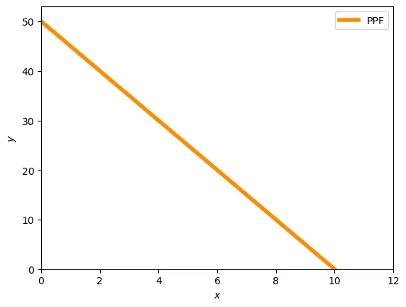
The economy can produce on any point on the PPF (also inside it). Exercise: show that producing inside the PPF does not use the entire labour force.

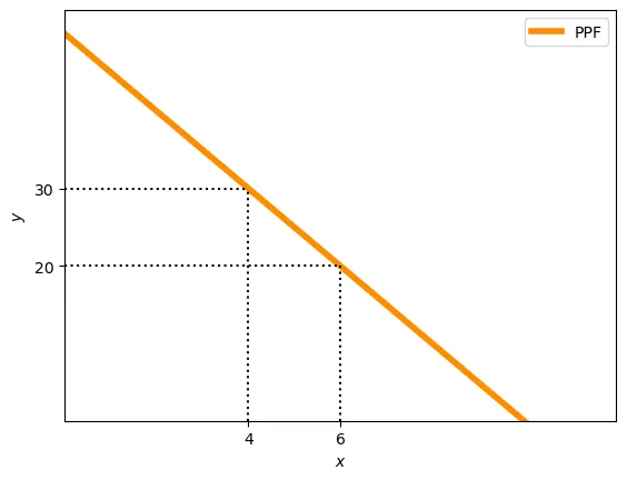
For instance, below we indicate several combinations of xbox and yogurts that are feasible:

1. 4 xbox and 30 yogurt
2. 6 xbox and 20 yogurt

Home country

Autarky equilibrium

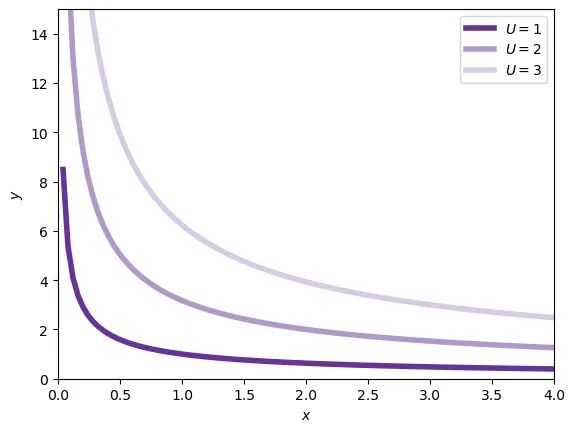
The economy can produce anywhere on the PPF. The exact production schedule will depend on the preferences of the consumers. Let’s suppose that consumers at Home have preferences described by a utility function such that: \begin{equation} U = u(x,y) \end{equation} For instance, $U = x^{0.4} y^{0.6}$ is a possible utility function (of the Cobb-Douglas family). If an individual consumes $x = 1$ xbox and $y = 20$ yogurt, the utility that he obtains is $U = 10^{0.4} 20^{0.6} = 6.03$. Because we are working on the $(x,y)$ space, we can plot the utility function as a curve called indifferece curve. The indifference curve plots all the points $(x,y)$ that provide the same level of utility $\bar{u}$. The next figure plots several indifference curves for the utility function $U = x^{0.4} y^{0.6}$.

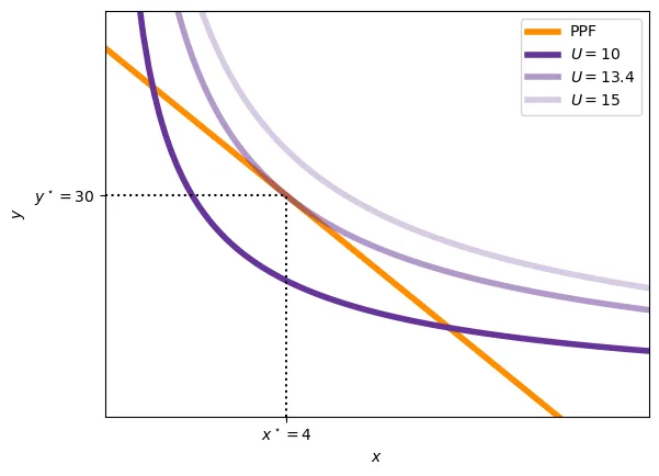
In autarky, the economy will produce at the point where the indifference curve is tangent to the PPF. We can show this mathematically. First, we must realize that consumers will want to maximize their utility. Second, that the production possibilities are limited by the PPF. Hence: \begin{align} \max_{x,y} U &= u(x,y) \\ \text{s.t.} \quad z_x x + z_y y &= L \\ \\ \max_x & \quad u(x, \frac{L - z_x x}{z_y}) \\ \frac{\partial u}{\partial x} &= 0 \implies \\ u^\prime_x - u^\prime_y \frac{z_x}{z_y} &= 0 \implies \\ \frac{u^\prime_x}{u^\prime_y} &= \frac{z_x}{z_y} \end{align} The term $-\frac{u^\prime_x}{u^\prime_y}$ is called the marginal rate of substitution and corresponds to the slope of the indifference curve. We can check this because: \begin{align} U &= u(x,y) \implies \\ 0 &= u^\prime_x dx + u^\prime_y dy \implies \\ \frac{dy}{dx} &= -\frac{u^\prime_x}{u^\prime_y} \end{align}

Hence, the slope of the PPF is $- \frac{z_x}{z_y}$ and the slope of the indifference curve is $-\frac{u^\prime_x}{u^\prime_y}$. The optimization problem will be solved when both slopes are equal, this is, when the indifference curve is tangent to the PPF.

Graphically:

Equilibrium relative price

Finally, the relative equilibrium price level that supports the autarky optimum. Within each industry, the wage of a worker is equal to the marginal product of labour. With a profit function of the type: \begin{equation} \pi_x = p_x x - w_x z_x x \end{equation} The profit maximizing condition is $p_x = w_x z_x$. Hence, the wage is $w_x = \frac{p_x}{z_x}$. The same applies to the yogurt industry, $w_y = \frac{p_y}{z_y}$.

Because workers can move freely between industries, the wage in both industries must be equal. Otherwise, workers would move from the industry with the highest wage to the industry with the lowest wage. Therefore, $w_x = w_y$ and $\frac{p_x}{z_x} = \frac{p_y}{z_y}$. And \begin{equation} \frac{p_x}{p_y} = \frac{z_x}{z_y} \end{equation} This is the ratio of the marginal productivities of labour: \begin{equation} \frac{p_x}{p_y} = \frac{z_x}{z_y} = \frac{MPL_y}{MPL_x} = \frac{\frac{1}{z_y}}{\frac{1}{z_x}} = \frac{z_x}{z_y} \end{equation}

If we let $z_x = 10$ and $z_y = 2$, then the equilibrium price ratio is $\frac{p_x}{p_y} = \frac{z_x}{z_y} = \frac{10}{2} = 5$.

Introducing the Foreign country

Similar to Home, the Foreign country will also have 2 industries, but with different marginal productivities of labour. Let’s suppose that in Foreign, 20 workers are needed to assemble an xbox and 6 workers are required to produce a yogurt. Hence, $z_x^\star = 20$ and $z_y^\star = 6$.

Absolute adavantage

We say that a country has an absolute advantage in the production of a good if producing this good requires less labour than in the other country. In our example, Home has an absolute advantage in the production of both goods: $z_x = 10 < z_x^\star = 20$ and $z_y = 2 < z_y^\star = 6$. This is, Home is more productive. Note that a country can have an absolute advantage in the production of more than one good.

Comparative advantage

Contrary to absolute advantage, comparative advantage is a relative concept. It compares the opportunity cost of producing a good across countries. A country with a lower opporunity cost has a comparative advantage in the production of that good.

In our example, $z_x = 10$ and $z_y = 2$ and $z_x^\star = 20$ and $z_y^\star = 6$. Therefore, the opportunity cost of one xbox at home is $\frac{z_x}{z_y} = \frac{10}{2} = 5$ yogurts. Meanwhile, the opportunity cost of 1 xbox in Foreign is $\frac{z_x^\star}{z_y^\star} = \frac{20}{6} = \frac{10}{3} \approx 3.33$ yogurts. Hence, Foreign has a comparative advantage in the production of xboxes because it has to give up less yogurts to produce an xbox.

Likewise, the opportunity cost of one yogurt at home is $\frac{z_y}{z_x} = \frac{2}{10} = 0.2$ xboxes. The same 1 yogurt in Foreign costs $\frac{z_y^\star}{z_x^\star} = \frac{6}{20} = 0.3$ xboxes. Consequently, Home has a comparative advantage in the production of yogurts.

In fact, with two countries and two goods, if one country has a comparative advantage in the production of one good, then the other country must have a comparative advantage in the production of the other good. \begin{equation} \frac{z_x}{z_y} < \frac{z_x^\star}{z_y^\star} \implies \frac{z_y}{z_x} > \frac{z_y^\star}{z_x^\star} \end{equation}

A complex example

The textile industry in the US generates 92000 USD per worker per hour while in China a similar worker generates only 13500 USD per hour. Meanwhile, a worker in the agricultural sector produces about 540 kg per hour and only 2 kg per hour in China. Note that we are given marginal productivities: if we add one more worker, we generate 92000 USD.

It is clear that the USA has an absolute advantage in both sectors: one worker generates more revenue in textiles and produces more per hour in agriculture. In fact, textiles workers are about 6.8 times more productive in the USA and farmers are 270 times more productive.

Let’s compute the opportunity cost of textiles in both countries. To produce one additional dollar in textiles we need $\frac{1}{92000}$ additional workers. This additional workers could have produced $540\frac{1}{92000} = 0.005$ kg. In China, it amounts to $2\frac{1}{13500} = 0.00015$ kg. Hence, the opportunity cost of textiles is lower than in the USA.

Specialisation and Trade

Similar to how we solved for the relative price level at Home, the relative equilibrium price level in Foreign is $\frac{p_x^\star}{p_y^s\star} = \frac{z_x^\star}{z_y^\star}$. In our example $\frac{p_x^\star}{p_y^\star} = \frac{20}{6} = \frac{10}{3} \approx 3.33$.

With this differential in relative prices, if we allow trade, an arbitrage opportunity will arise. We can borrow one hundred yogurts in Home, sell it in Foreign and obtain $\frac{100}{\frac{p_x^\star}{p_y^\star}} = 30$ xbox Then, back at Home, $30$ xboxes can be exchanged for $30 \times 5 = 150$ yogurts. We can return the 100 we borrowed and still gain 50.

Someone will start exploiting this possibility. Because the supply of xboxes in Home increases, the relative price of xboxes will fall. At the same time, the demand of xboxes in Foreign increases, driving up its price.

In other terms, Home exports yogurt and imports xboxes. The flow of goods will stop once the relative prices in both countries are equal.

We do not know yet towards which price level the world will converge to. However, the world equilibrium price level must be between the relative price levels of the two countries:

\begin{equation} \left(\frac{p_x}{p_y}\right)^\star < \left(\frac{p_x}{p_y}\right)^w < \frac{p_x}{p_y} \end{equation}

To see why, suppose it is not, for instance, assume that $\left(\frac{p_x}{p_y}\right)^w = 1$ Because the world price of xboxes is lower than the Home price of xboxes, Home would one to import them. However, the world price is also lower than the price at Foreign, so that Foreign also wants to import xboxes. This is impossible, because none will be exporting any!

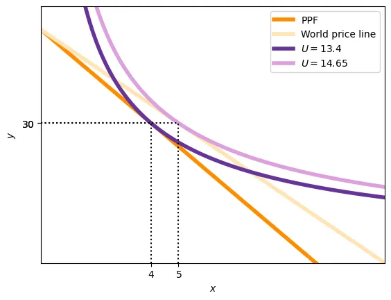
The next natural question is whether Home and Foreign benefit from trading at the world price. The answer is yes, and we can see it graphically.

For the sake of the argument, assume that $\left(\frac{p_x}{p_y}\right)^w = 4$ Home can gain if the country specializes in yogurts. With a working force of $L = 100$, it can produce $50$ yogurts. These $50$ yogurts can be exchanged for 12.5 xboxes, meaning that the budget constraint has shifted. In fact, it is no longer the case that consumption must be tangent to the PPF: international trade expands the consuption set beyond the PPF. With the previous utility function $U = x^{0.4}y^{0.6}$, the optimum is to consume: \begin{align} \max_{x,y} U &= x^{0.4}y^{0.6} \\ \text{s.t. } & 50 p_y = y p_y + x p_x \implies 50 = y + \frac{p_x}{p_y} x \implies y = 50 - 4 x \\ \\ x &= 5 \quad y = 30 \end{align}

Home will consume more of both goods than before (actually, in this example it is the same amount of yogurt, but it needs not be the case).

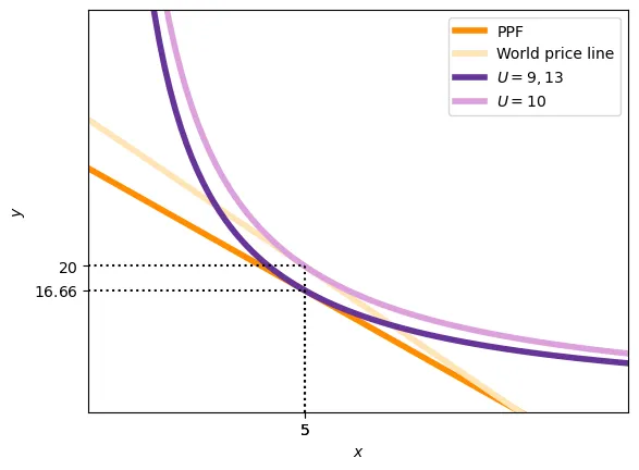
With a utility function $U = x^{0.5} y^{0.5}$ and a work force of $L^\star = 200$, in autarky, Foreign consumption was: \begin{align} \max_{x,y} U &= x^{0.5}y^{0.5} \\ \text{s.t. } & L^\star = 20 x + 6 y \\ x &= 5 \quad y = 16.67 \end{align}

Because the xboxes are produced in Foreign, the 5 imported at Home require 100 workers. The remaining 100 workers can produce the 5 xboxes that were consumed in Foreign under autarky. Moreover, the 5 exported xboxes will be exchanged for 20 yogurts, more than what they consumed in autarky, so Foreign is better off under trade.

Pattern of trade

The general conclusion of Ricardo’s model is that countries should specialize in the good for which they have a comparative advantage, producing and exporting it. The good that is exported is traded against the good for which the country has a comparative disadvantage, which is imported.

In that sense, according to Ricardo’s model, the pattern of trade is determined by comparative advantage.

Moreover, as we have seen with the example, international trade expands the consumption set, improving the well-being of both countries. In that sense, trade is Pareto-improving: every country wins, none looses.

Wages

However, many opponents to international trade argue that, by importing a good, workers in that sector suffer. For instance, one could claim that Home xbox producers suffer because Home specialized in yogurt.

Even with trade, firms are still working under perfect competition. Therefore, the wage in each sector and country still corresponds to the marginal product of labor. Because Home produces yogurts and Foreign xboxes: \begin{align} w_y &= p_y MPL_y \\ w_x^\star &= p_x MPL_x^\star \end{align} Note that prices are common due to trade.

The xbox industry disappeared at Home, why? The answer is simple: no one wants to work in that industry. In autarky, wages were equal in both sectors with $w_x = p_x MPL_x$ and $w_y = p_y MPL_y$. Hence $\frac{w_x}{w_y} = 1$.

In autarky, we also had $\frac{p_x}{p_y} = \frac{MPL_y}{MPL_x}$. But, with trade $\left(\frac{p_x}{p_y}\right)^w < \frac{MPL_y}{MPL_x}$ so: $p_x^w MPL_x < p_y^w MPL_y$ Because wages are the marginal products: $\frac{w_x}{w_y} = \frac{p_x^w MPL_x}{p_y^w MPL_y} < 1$ and a worker at Home earns more in the yogurt sector. As a consequence, the xbox sector disappears at Home whenever the relative price xboxes is lower than in autarky. Similarly, the yogurt industry disappears in Foreign.

The wage at Home is $w_y = p_y MPL_y$ and the wage at Foreign is $w_x^\star = p_x MPL_x^\star$. Consequently, wages at Home are higher if:

• $p_y MPL_y > p_x MPL_x^\star$ (wages measured in dollars)
• $MPL_y > \frac{p_x}{p_y} MPL_x^\star$ (wages measured in yogurts)
• $\frac{p_y}{p_x} MPL_y > MPL_x^\star$ (wages measured in xboxes)

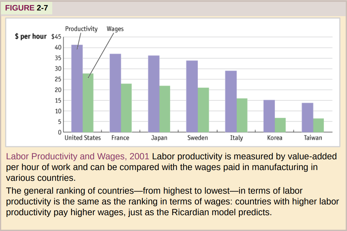
Therefore, wages are determined by the absolute advantage: higher productivity translates as higher wages (ignoring for a second the price level which we do not know how to determine).

International prices

The last piece to close the model is the determination of the international price level. Again, remember that we will find a relative price $\frac{p_x}{p_y}$.

As always in economics, we first need to find the supply and demand curves. In general, when dealing with trade, one looks for a relative supply and relative demand curve. However, for the Ricardian model, we can work out the equilibrium price by stuyding just one market. The budget constraint (total production equals total consumption) will ensure that the other market is also in equilibrium.

Supply of exports

Let’s consider Home. If the international price ratio $\left(\frac{p_x}{p_y}\right)^w$ is smaller than $\frac{p_x}{p_y} = \frac{z_x}{z_y}$ in autarky, Home specializes in yogurts. When the international price ratio equals the one prevailing in autarky, Home is indifferent between producing xboxes or yogurts. Finally, when $\left(\frac{p_x}{p_y}\right)^w > \frac{z_x}{z_y}$, Home specializes in xboxes.

In our example, we had that $\frac{z_x}{z_y} > \frac{z_x^\star}{z_y^\star}$ so that Home specializes in yogurts. The production of yogurts is then $y = \frac{L}{z_y}$. Out of the amount produced, some will consumed internally and some exported. Internal consumption can be retrieved from the utility maximization.

\begin{align} \max_{x,y} & \ u(x,y) \\ \text{s.t.} & \ p_x x + p_y y = p_y \frac{L}{z_y} \\ \\ \max_{x,y} & \ u(x,y) \\ \text{s.t.} & \ \frac{p_x}{p_y} x + y = \frac{L}{z_y} \implies \\ \max_{y} & \ u\left(\frac{\frac{L}{z_y} - y}{\frac{p_x}{p_y}}, y\right) \\ u^\prime_x \frac{1}{\frac{p_x}{p_y}} = u^\prime_y \implies \\ \frac{u^\prime_x}{u^\prime_y} = \frac{p_x}{p_y} \end{align}

Then, if $u(x,y) = x^{0.4}y^{0.6}$ with $L=100,\ z_x = 10, z_y = 2$ \begin{align} \max_{x,y} & \ x^{0.4}y^{0.6} \\ \text{s.t.} & \ \frac{p_x}{p_y} x + y = 50 \\ \\ y = 30 \end{align}

Note that, for this specific utility function, the optimal consumption of yogurts is independent of the price ratio. In general, this is not the case.

Then, the supply of exports is $y^\text{prod.} - y^\text{cons.} = 50 - 30 = 20$.

Demand of imports

Demand of imports (of yogurts) comes from Foreign. If we assume they specialize in xboxes, then they produce $\frac{L^\star}{z_x^\star} = 10$ xboxes. Their budget constraint is $p_x x + p_y y = p_x^\star \frac{L^\star}{z_x^\star} p_x = 10 p_x$. With preferences represented by $u = x^{0.5}y^{0.5}$, the demand of yogurts is given by: \begin{align} \max_{x,y} & \ x^{0.5}y^{0.5} \\ \text{s.t.} & \ p_x x + p_y y = 10 p_x equiv \frac{p_x}{p_y} x + y = 10 \frac{p_x}{p_y} \\ \max_{y} & \ \left(\frac{10 \frac{p_x}{p_y} - y}{\frac{p_x}{p_y}}\right)^{0.5} y^{0.5} \\ y = 5 \frac{p_x}{p_y} \end{align}

So, the demand of yogurts is $5 \frac{p_x}{p_y}$.

Equilibrium

The equilibrium is given by the intersection of the supply and demand curves. In our example: $20 = 5 \frac{p_x}{p_y} \implies \frac{p_x}{p_y} = 4$

Changes in the international price and gains from trade

We know already that both countries gain from trade. However, it is likely that one country gains more than the other. We can analyze the relative gains by analyzing what happens when the price changes.

In our baseline example, Home exports yogurt and imports xboxes. This means that Home gains $p_y$ whenever a yogurt is exported and pays $p_x$ whenever an xbox is imported. Therefore, if $p_y$ increases, Home gains more. Similarly, if $p_x$ increases, Home gains less from trade. In general, we define the terms of trade as the ratio between the price of the exported good divided by the price of the imported good. For Home that exports yogurts, the terms of trade are $T = \frac{p_y}{p_x}$.

When does Home gain more from trade? Let’s analyze several changes that may occur.

Home becomes more productive in yogurts

To simplify a bit the notation, let $p \equiv \frac{p_x}{p_y}$. This means that $z_y$ decreases. Because of the specialization of Home in yogurts, and using the previously derived demand and supply, we will have that internal demand for yogurts solves $\frac{u^\prime_x}{u^\prime_y} = p$, remaining the same. At the same time, the production $\frac{L}{z_y}$ increases. Therefore, the supply curve shifts to the right, increasing. Because the demand from Foreign has not changed, the price $p = \frac{p_x}{p_y}$ falls. This makes Home worse off, because it exports yogurts at a lower price. Note: with the caveat that Home is producing and exporting more, so perhaps the larger exports compensate the drop in prices.

Home becomes more populated

Similar to before, an increase in $L$ will translate as an increase in the supply of yogurts, because $\frac{L}{z_y}$ increases. This will make the price of yogurts fall, making Home worse off.

Because of the pattern we have just seen, in general larger and more productive countries will gain less from trade. To think about it, it is just as if they had been growing over time and thus eroding little by little their terms of trade. Alternatively, one can say that it is smaller and less productive countries that gain more.

Equilibrium without full specialization

The Ricardian model allows for the case where one (and only one) country does not fully specialize in any good. This is, under some circumstances, a country will produce both goods, while its trading partner will specialize in one.

For one country not to specialize, it must be the case that the international price equals the price that would prevail under autarky, so that it is indifferent. This also means that the equilibrium price ratio must coincide with $\frac{z_x}{z_y}$.

Let’s take the previous case with Home specialized in yogurts. If the size of Home increases $L \uparrow$, then the price $\frac{p_x}{p_y}$ will raise from the equilibrium 4 up to a maximum of $\frac{z_x}{z_y} = \frac{10}{2} = 5$ as $p_y$ falls due to the increase in supply. Therefore, non-specialization can occur when one country is much larger than the other. Also, because $\frac{p_x}{p_y}$ also increases when Home becomes more productive in yogurts, non-specialization can occur when one country is much more productive than the other.

We can also see this in reverse. When Home is much larger than Foreign, it can be the case that even when all Foreign workers are engaged in the production of the good they export (xboxes) their production is not enough to satisfy the demand of Home. In this case, Home will produce some of the good it imports (xboxes) and export the other (yogurts).

Example

Let $L=1000$ instead of 100 as before, while keeping $z_x = 10$ and $z_y = 2$. With the utility we had before, the supply of yogurts for export is $\frac{L}{z_y} - 30 = 470$ under full specialization. With a demand from Foreign equal to $5 \frac{p_x}{p_y}$, the equilibrium price would be $\frac{p_x}{p_y} = 94$. Clearly, the “equilibrium” price is above the autarky price, and Home would prefer not to trade at this price level.

Instead, Home will produce both goods and trade at the least favorable price level: $\frac{p_x}{p_y} = \frac{z_x}{z_y} = 5$. At this price point, Foreign demand of yogurts is $5 \frac{p_x}{p_y} = 25$. For the 25 yogurts, Home will receive 5 xboxes. At this price ratio, Home will consume: \begin{align} \max_{x,y} & u(x,y) = x^{0.4}y^{0.6} \\ \text{s.t.} & 1000 = 10 x + 2 y \\ \\ x = 40, y = 300 \end{align} Thus, Home will produce 325 yogurts (300 for consumption and 25 for the export market) and 35 xboxes.

It is clear that Home will remain in the autarky schedule, thus not benefiting from trade. However, Foreign will still gain from trade because it has access to a price ratio of $5$ when the opportunity cost they have is 3.33.

Beyond Ricardo

• Dornbush, Fisher and Samuelson (1977): Generalizes Ricardo with many goods
• Eaton and Kortum (2002): Generalizes Dornbush, Fisher and Samuelson (1977) with many countries and trade costs. It is a popular trade model and the basis from master studies in trade.

Exercises

Note: Exercises 1, 2 and 3 provide an alternative way to solve the model.

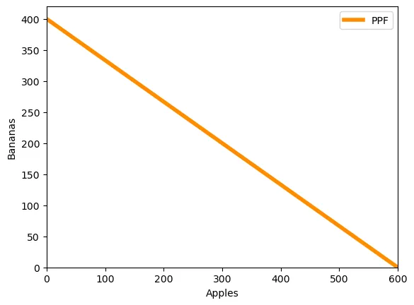
1. Home has 1200 units of labor available. It can produce two goods, apples and bananas. The unit labor requirement in apple production is 3, while in banana production it is 2.

   1. Plot Home’s PPF (bananas on x-axis)

      

   2. What is the opportunity cost of apples in terms of bananas? The opportunity cost of appes in terms of bananas can be computed as $\frac{z_a}{z_b} = \frac{3 \frac{\text{workers}}{\text{apple}}}{2 \frac{\text{workers}}{\text{banana}}} = \frac{3}{2} \frac{\text{banana}}{\text{apple}}$. This reflects that producing 1 apple requires 3 workers. To increase 1 apple’s production by 1, we need 3 additional workers. With 3 workers one can harves $\frac{3}{2}$ bananas.

   3. In the absence of trade, what would be the price of apples in terms of bananas? Why? With labour mobility, the wage has to be the same in both sectors. Moreover, with perfect competition, wages are the marginal productivity. Hence: $w_a = p_a \frac{1}{3}$ and $w_b = p_b \frac{1}{2}$. Setting $w = w_a = w_b$ gives us $\frac{p_a}{p_b} = \frac{3}{2}$.

2. There is now also another country, Foreign, with a labor force of 800. Foreign’s unit labor requirement in apple production is 5, while in banana production it is 1.

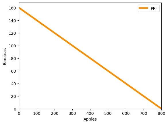
   1. Graph Foreign’s production possibility frontier.

      

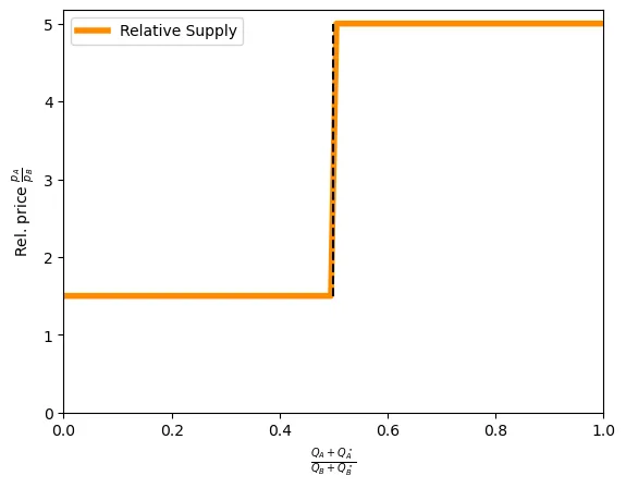
   2. Construct the world relative supply curve. Note: this technique was not explained in the course. The autarky price of apples in terms of bananas in Foreign is $\frac{p_a}{p_b} = \frac{5}{1} = 5$. Hence, Home will specialize in apples and Foreign in bananas. The relative supply curve indicates the total supply of apples divided by the total supply of bananas, considering both countries. Suppose the international price level is 1.5. At this price level, Home is indifferent between trading or not, while Foreign specializes in bananas. The minimum number of apples that Home can produce is 0, and the maximum is $\frac{L}{z_a} = \frac{1200}{3} = 400$. With Foreign specializing in bananas, it will produce 0 apples and 800 bananas. Hence, at price level $\frac{3}{2}$ the world relative supply of apples takes values between $\frac{0}{800}$ and $\frac{400}{800}$. For prices between $\frac{3}{2}$ and $5$, each country specializes in one good: Home produces 400 apples and 0 bananas, while Foreign produces 0 apples and 800 bananas. Hence, the world relative supply is $\frac{400}{800} = \frac{1}{2}$ for $1.5 \leq \frac{p_a}{p_b} \leq 5$. At price $5$ and above, both countries specialize in apples. Hence, the relative supply of apples goes to infinity. Graphically:

      

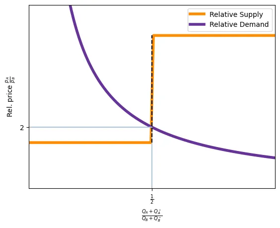
   3. Assuming that the world relative demand for apples is $\frac{D^A}{D^B} = \frac{p_b}{p_a}$, find the equilibrium price and plot it.

   When $\frac{p_a}{p_b} = 2$, the relative demand is 2, which is a point on the relative supply schedule, revealing the equilibrium.

   

3. Home is characterized by $L = 50, z_x = 4, z_y = 1$, where $z_{i}$ indicates number of workers required to produce one unit. Consumer preferences are given by $u(x,y) = \log(x) + y$ (log-linear preferences, non-homothetic).

   1. What is the autarky wage? Because labor is mobile across sectors, the wage must be equal in both. A firm maximizes profits $\pi_x = p_x x - w_x z_x x \implies w_z = w = \frac{p_x}{z_x}$. Similarly, $w_y = w = \frac{p_y}{z_y}$.

   2. What is the autarky price ratio? From the condition above, $w = \frac{p_x}{z_x} = \frac{p_y}{z_y} \implies \frac{p_x}{p_y} = \frac{z_x}{z_y} = 4$. We will come back to this later.

   3. What is the autarky production and consumption? In autarky, production equals consumption all while maximizing utility. \begin{align} \max_{x,y} \log(x) + y \\ \text{s.t.} & 50 = 4 x + y \\ \\ x = 0.25, y = 49 \end{align}

   4. Suppose that Foreign has $L^\star = 60$ workers, technology $z_x^\star = 6$ and $z_y^\star = 2$. Utility is $u(x,y) = \log(x) + \log(y)$. According to the Ricardian model, which good will Home export? The opportunity cost of $x$ in Home is $\frac{z_x}{z_y} = 4$ and in Foreign is $\frac{z_x^\star}{z_y^\star} = 3$. Hence, Home has a comparative advantage in $y$ and will export $y$ and import $x$.

   5. For which price range both countries will specialize in only one good? As long as $3 < \frac{p_x}{p_y} < 4$, both countries will specialize in only one good.

   6. Determine the equilibrium relative price and the exports and imports. Because Home exports $y$, we construct the international supply of $y$ as a function of $\frac{p_x}{p_y}$ Assuming a full specialization, Home will produce $\frac{L}{z_y} = 50$ units of $y$. The internal demand is: \begin{align} \max_{x,y} u= & \log(x) + y \\ \text{s.t.} & 50 p_y = p_x x + p_y y \implies 50 = \frac{p_x}{p_y} + y \\ \\ \max_{y} & \log\left(\frac{50-y}{p_x}\right) + y \\ y &= 49 \end{align} Hence, the international supply of $y$ is 1 unit, regardless of prices.

      We assume that foreign specializes in $x$, producing $\frac{L^\star}{z_x^\star} = 10$ units of $x$. The demand function for $y$ from Foreign comes from: \begin{align} \max_{x,y} u &= \log(x) + \log(y) \\ \text{s.t.} & 10 p_x = p_x x + p_y y \implies 10 \frac{p_x}{p_y} = x \frac{p_x}{p_y} + y \\ \\ \max_{y} & \log\left(\frac{10\frac{p_x}{p_y}-y}{\frac{p_x}{p_y}}\right) + \log(y) \\ y &= 5\frac{p_x}{p_y} \end{align}

      Hence, the international demand for $y$ is $5\frac{p_x}{p_y}$ and the equilibrium price is $1 = 5 \frac{p_x}{p_y} \implies \frac{p_x}{p_y} = \frac{1}{5}$.

      Such a price cannot be an international equilibrium because Foreign, which has a comparative advantage in $x$, displays an opportunity cost for that good equal to 3. Consequently, Foreign will produce both $x$ and $y$ while Home will specialize in $y$, with an international price $\frac{p_x}{p_y} = 3$. Home has a demand of $y$ equal to 49 (independent of the price). Because Home specializes, all the 50 workers are employed in $y$ production, generating $\frac{L}{z_y} = 50$ units of $y$. Hence, Home will export 1 unit of $y$. At the ongoing price $\frac{p_x}{p_y} = 3$, Home will exchange this 1 unit of $y$ for 0.33 units of $x$, thus Home is better off than under autarky. Meanwhile, Foreign consume 15 units of $y$ ($5 \frac{p_x}{p_y} = 15$), of which 14 are locally produced requiring 28 workers. The remaining 32 are employed in the $x$ sector, generating 5.33 units. Hence, total consumption of $x$ in Foreign is $5.33-0.33=5$ units. We can check that this coincides with the autarky consumption levels in Foreign: \begin{align} \max_{x,y} u &= \log(x) + \log(y) \\ \text{s.t.} & 60 = 6x + 2y \\ \\ \max_{x} & \log(x) + \log\left(\frac{60-6x}{2}\right) \\ x &= 5, y = 15 \end{align}

      Note: in this exercise, the equilibrium price of $0.2$ mostly came from the fact that Home had a very large demand for $y$.