Empirics around Ricardo

Introduction

The Ricardian model of international trade is simple and provides a clear prediction about the pattern of trade between countries.

1. Countries should specialize in the good in which they have a comparative advantage.
2. With free trade, a country that exports a good does so at a (relative) price level higher than under autarky. Otherwise, it would not export it!

For instance, if we have two countries with: \begin{equation} \frac{z_x}{z_y} > \frac{z_x^\star}{z_y^\star} \end{equation} Then the opportunity cost of producing good $x$ is higher at Home than in Foreign. Consequently, Home should specialize in good $y$, Foreign in good $x$ and trade.

How can we test the specialization patterns using data? The takeaway of the Ricardian model “a country will specialize (and export) the goods for which it has a relative high productivity, and import the goods for which it has a relative low productivity” Notice the change from opportunity cost and labor requirements to productivity!

If we had data on productivity for all goods and production (or trade data), the exercise would be simple: just correlate the two. The main problem with this approach is that the data we have does not provide all we need:

• Prices: yes
• Who produces what and quantities: yes
• Unitary labor costs (or labor requirements) for the produced good: maybe

The issue is that we do not observe the productivity (or labor costs, or labor requirements) of the goods that are not produced. “The difference in labor requirements cannot be observed, since imported goods will almost never be produced in the importing country.” (Deardorff, 1984)

Costinot and Donaldson (2012)

Costinot and Donaldson (2012) proposed to use the agricultural sector because the productivity of a given crop under different circumstances is very well studied. Indeed, GAEZ (Global Agro-Ecological Zones) project by the FAO predicts the productivity of land for the entire planet and for several crops. With these data, we can very easily get a sense of how many kg of tomaotes can be produced per hectare in a given region. To do this, the GAEZ relates soil characteristics, elevation, water availability, insolation, temperatures, etc. to the growing cycle of each plant using agricultural models.

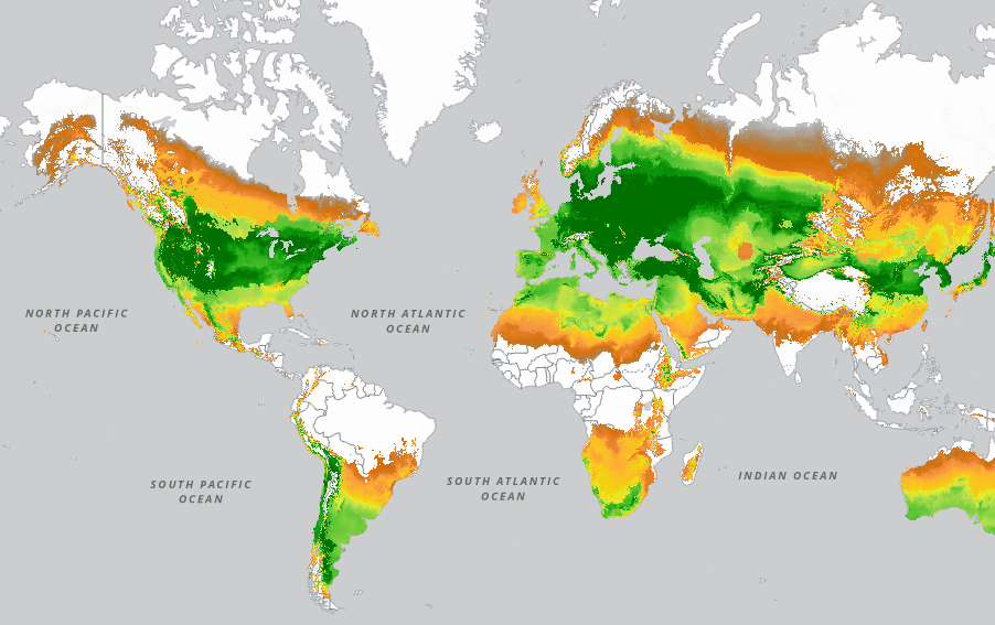
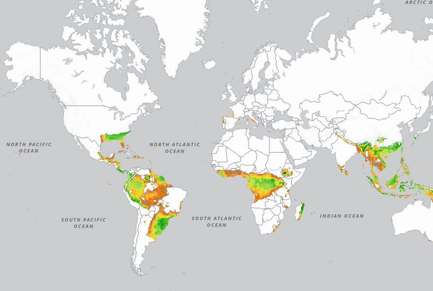
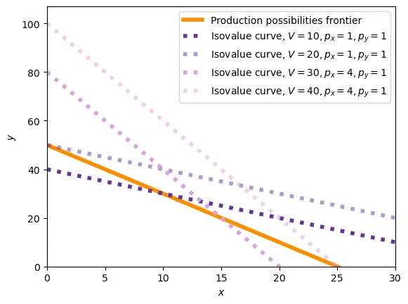
Suppose France has 10 fields $f$ on which three crops can be grown: wheat, bananas and grapes. The productivity of each crop in each field is known thanks to GAEZ. The problem then boils down to selecting the crops that yield the largest value in each field. It is important to note here that the yield value depends both on the prices and the productivity of each field in each crop. A simple GDP maximization problem can be written as: \begin{align} \max_{K^i_{f}} & \sum_{f=1}^{10} \sum_{i=1}^{3} p_i K^i_{f} y_{f}^i \\ \text{s.t} & \sum_{i=1}^{3} K^i_{f} = 1, \forall f=1, \dots, 10 \\ & K^i_{f} \in \{0,1\}, \forall f=1, \dots, 10, \forall i=1, \dots, 3 \end{align} where $p_i$ is the price of crop $i$, $y_{f}^i$ is the productivity of crop $i$ in field $f$ and $K^i_{f}$ indicates whether crop $i$ produced in field $f$ or not. The restrictions simply state obvious constraints: $\sum_{i=1}^{3} K^i_{f} = 1$ indicates that a field must be fully used, while $K^i_{f=j} \in \{0,1\}$ indicates that a field can only produce one crop, so each field has to be used with one and only one crop. Without entering into the details, this is a linear progamming problem that can be solved using the simplex method. But a more intuitive way to solve this problem is to sort the crops by the yield value (productivity time price) in each field and then select the crops with the highest value.

Detour

If we go back to Ricardo’s model, we can show that what we just described corresponds to the production decision, even though we are not limited to producing only one unit of a good. Assume that we are given prices, then a country will specialize as follows: \begin{align} \max_{x,y} & p_x x + p_y y \\ \text{s.t.} & z_x x + z_y y = L \\ & x, y \geq 0 \\ \end{align}

The solution to the above problem is: $\{x = \frac{L}{z_x}, y = 0\} \ \text{if}\ \frac{p_x}{p_y} > \frac{z_x}{z_y}$ and $\{x = 0, y = \frac{L}{z_y} \} \ \text{if}\ \frac{p_x}{p_y} < \frac{z_x}{z_y}$. This is, when the relative price of $x$ is higher than the relative productivity of $x$, then the country will specialize in $x$ and vice versa.

Using the method we described, Costinot and Donaldson can compute the crop that maximizes yields for each field in each country. Then, by aggregating predicted production (using the GAEZ data) over all the fields in a country, they can compute the production of each crop in each country. Finally, they compare the prediction based on comparative advantage from Ricardo’s model to the actual production data.

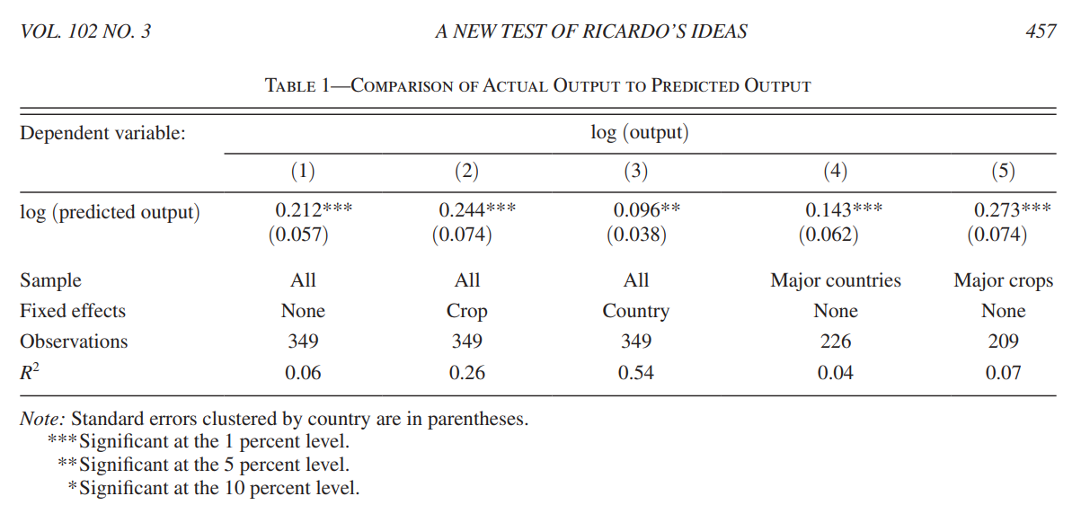
They find a positive correlation between the predicted production (in logaithms) and the actual production (in logarithms). The coefficient is not 1 (as it should if the model were perfect) because the only land uses they considered are for farming, yet land is also used for other purposes: urban areas, industrrial areas, infastructure, etc. Another problem is that the data from GAEZ divides the world in squares of approximilately 10km by 10km. The best crop can vary within that area, so the model might not be able to capture that.

All-in-all, the model does a good job at predicting the production of each country, but it is not perfect:

We have asked a simple question: How do output levels predicted by Ricardo’s theory compare to those that are observed in the data? Despite all of the real-world considerations from which Ricardo’s theory abstracts, we find that a regression of log output on log predicted output has a (precisely estimated) slope of 0.21. Ricardo’s theory of comparative advantage, is not just mathematically correct and nontrivial; it also has significant explanatory power in the data, at least within the scope of our analysis.

Bernhofen and Brown (2004)

Costinot and Donaldson (2012) show that, given prices, productivities are quite good at predicting patterns of specialization. This is, we have empirically validated that countries tend to specialize in the good that they are more productive in (lower unitary requirements). However, the Ricardian model is mostly about trade. The main prediction in that sense is that free trade causes a country to export the good in which it has a comparative advantage.

Extending this result, a natural corollary arises: because a country tends to specialize in the good for which it has a comparative advantage, it means it can produce this good more cheaply than other countries. Put it in other terms: to sell that good, the international price must be higher than the domestic opportunity cost. Since prices in autarky reflect the domestic opportunity cost, it follows that the international price must be higher than the autarky price.

The problem is that, in general, one does not observe the same country in autarky and under free trade. Bernofen and Brown (2004) lookd at Japan, which opened itself to trade in 1853. From 1639, Japan forbid all contact with outsiders, isolating itself from international markets and operating under autarky. In 1853, Commodore Matthew Perry, an American naval officer, led a fleet of four warships to Japan in an attempt to force the country to open its ports to foreign trade. Japan had been under a strict policy of isolation for over 200 years, known as “sakoku,” which had prevented any contact with outsiders. By 1860, after several military interventions and treaties, Japan had opened its ports to foreign trade and began to modernize its economy.

Let’s have a look at the results from a comparison of price increases to pre-1853 trade levels:

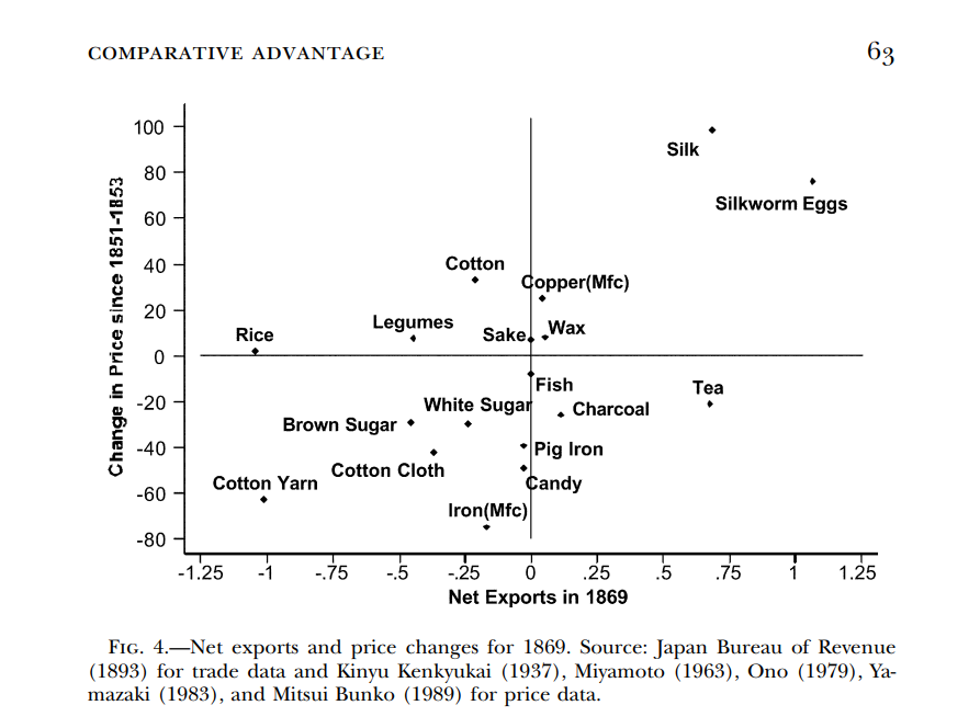
As the authors say:

The prices of major exports such as products of the silk industry (silk and silkworm eggs) and minor exports such as copper manufactures, sake, and vegetable wax all increased; in some cases they almost doubled. The relative price of key imports such as sugar, cotton cloth, cotton yarn, and iron products displayed substantial declines. The increase in the price of rice and legumes may reflect poor weather conditions, and the increase in the price of cotton may stem from the disruption of cotton markets in the wake of the American Civil War.

This corroborates the Ricardian model: Japan specializes in the good for which it has a comparative advantage, and because the international price is higher than the autarky price, once trade begins the price of the good increases.

A second test the authors implement is based on the same idea. Let’s work it out with an example:¹ Suppose that, under autarky with autarky prices ($p_x = 4, p_y = 8$), the country decides to consume (and produce!) at the levels $x = 50, y = 25$. Assume that international prices, one the country opens up to trade, are $p_x = 5, p_y = 5$. Because the country has a comparative advantage in $x$, it will export $x$ and import $y$. At this new price level, consumption is $x = 50, y = 50$, with the country using all its labor force to produce $x$.

When trade begins, the good we export becomes more expensive and the imported good cheaper. It is possible to show that the value of net exports (exports minus imports) evaluated at autarky prices is negative. In our example, the net export of $x$ is $50 - 0 = 50$ and the net export of $y$ is $0 - 50 = -50$. Thus, the value of net exports is $50 \times 4 + (-50) \times 8 = -200 < 0$.

We can show this more generally. When the economy opens up to international trade, in the Ricardian model trade is balanced, meaning that the value of exports equals the value of imports. Suppose that $\frac{p_x^f}{p_y^f} > \frac{p_x^a}{p_y^a}$, so that $x$ is the good with comparative advantage. Using $x$ and $y$ for production and $c_x$ and $c_y$ for consumption, we have: $p_x^{f} (x^f-c_x^f) = p_y^{f} (c_y^f-y^f)$, where $x^f - c_x^f > 0$ because the country exports $x$ and $c_y^f - y^f$ > 0, because the country imports $y$. The superscript $f$ denotes the free trade equilibrium. From here: \begin{align} p_x^{f} (x^f-c_x^f) &= p_y^{f} (c_y^f-y^f) \implies \\ \frac{p_x^{f}}{p_y^f} (x^f-c_x^f) &= (c_y^f-y^f) \implies \\ \frac{p_x^{f}}{p_y^f} (x^f-c_x^f) - (c_y^f-y^f) &= 0 \\ \frac{p_x^{f}}{p_y^f} (x^f-c_x^f) - (c_y^f-y^f) &> \frac{p_x^a}{p_y^a}(x^f-c_x^f) - (c_y^f-y^f) \implies \\ \frac{p_x^a}{p_y^a}(x^f-c_x^f) - (c_y^f-y^f) < 0 \end{align} Where $\frac{p_x^{f}}{p_y^f} (x^f-c_x^f) - (c_y^f-y^f) > \frac{p_x^a}{p_y^a}(x^f-c_x^f) - (c_y^f-y^f)$ is true because $\frac{p_x^{f}}{p_y^f} > \frac{p_x^a}{p_y^a}$.

The setup in Bernhofen and Brown is a bit more complex because they have more goods and trade may not be balanced. In any case, the general conclusion holds: if we evaluate net exports at autarky prices, we should observe a negative value.

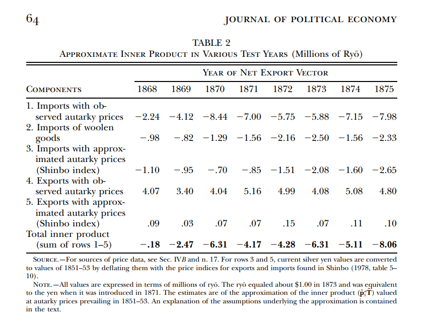
This is exactly the result, confirming again the validity of the Ricardian trade model. In this case, they have shown that trade patterns are in accordance with the theoretical predictions.