Debt and public expenditures

Based on de la Croix and Michel, Chapter 4.4

The Ricardian equivalence

The Ricardian equivalence states that forward-looking agents internalise the government’s budget constraint when deciding. Hence, whether public expenditures are financed using debt or taxes is irrelevant.

Intuitively, forward-looking agents —who shall live forever– know that, if the government increases expenditures today without raising taxes, debt will be issued and taxes eventually increased to pay it off.

However, as we shall see, in the OLG model, the Ricardian equivalence does not hold. Clearly, the main difference between the OLG and Ramsey models is that agents live only for two periods in the former. Suppose that the government decides to run a deficit today to increase public expenditures. Young and old individuals today are not that much affected because, when the government raises the taxes to pay the debt off, they would have already died. Instead, if the government decides to increase taxes today, it affects present-day young and old individuals.

The model with a government

The government

Suppose the government has public expenditures of $g_t$ per young individual. Total expenditures are then $G_t = N_t g_t.$ These public expenditures are financed by a lump-sum tax of $\tau_t$, which is paid only by the young. Total revenues are $T_t = N_t \tau_t.$ Finally, the government can have debt. The total outstanding debt is $B_t,$ and $b_t$ represents it per young terms. The government pays interest on the debt of the previous period: $R_t B_{t-1}.$

We can write the government’s budget constraint:

$$G_t + R_t B_{t-1} = B_t + T_t.$$

The constraint, expressed in per capita terms, is:

$$\frac{G_t}{N_t} + R_t \frac{B_{t-1}}{N_t} = \frac{B_t}{N_t} + \frac{T_t}{N_t} = $$ $$g_t + R_t \underbrace{\frac{B_{t-1}}{N_{t-1}}}_{b_{t-1}}\underbrace{\frac{N_{t-1}}{N_{t}}}_{\frac{1}{1+n}} = b_t + \tau_t = $$ $$g_t + R_t \frac{b_{t-1}}{1+n} = b_t + \tau_t $$

As a final note, government spending is unproductive: it does not affect the production function. Moreover, individuals do not derive utility from it. Finally, we assume that the government always honors its debt. In that sense, government debt is a riskless asset.

Individuals

The budget constraint of a young individual who now pays taxes $\tau_t$ is:

$$w_t = c_t + s_t + \tau_t$$ $$R_{t+1}s_t = d_{t+1}.$$

Alternatively, we can express it as an intertemporal budget constraint:

$$w_t = c_t + \tau_t +\frac{d_{t+1}}{R_{t+1}}.$$

We can easily obtain the savings function as we did before by substitution:

$$\max_{c_t, s_t, d_{t+1}} u(c_t) + \beta u(d_{t+1})$$ $$\mathrm{s.t.}, w_t = c_t + s_t - \tau_t$$ $$\phantom{\mathrm{s.t.}}, d_{t+1} = R_{t+1}s_t.$$

Then:

$$\max_{s_t} u(w_t-s_t-\tau_t) + \beta u(R_{t+1}s_t).$$

The first order condition reads:

$$u^\prime(w_t - s_t-\tau_t) = \beta R_{t+1} u^\prime(R_{t+1}s_t).$$

From here, we can recover the savings function:

$$s_t = s(w_t-\tau_t, R_{t+1}).$$

In this model, households have access to two types of savings:

• savings in capital
• and government bonds.

Moreover, the risk of both types of investment is the same: none, because both assets are riskless. Hence, bonds and capital are perfect substitutes. in the portfolio of wealth owners.¹ Therefore, the entire amount households decide to save is split between the two

$$N_t s_t = K_{t+1} + N_t b_t.$$

Equilibrium

At the (temporal) equilibrium , the government chooses $B_t, \tau_t$ to satisfy its budget constraint: $g_t + R_t \frac{b_{t-1}}{1+n} = b_t + \tau_t.$ Moreover, as we have already discussed, because debt and capital are substitutes, both bear the same interest $R.$ Also, firms operate in a perfectly competitive environment and factors are paid their marginal productivities:

$$w_t = \omega(k_t)$$

and $$R\_t = f^\prime(k\_t)$$ with $k\_t \equiv \frac{K\_t}{N\_t}.$

Introducing this into the government budget constraint we obtain:

$$B_t + N_t \tau_t = G_t + f^\prime(\color{red}{k_t})B_{t-1}.$$

We have implicitly assumed that investment is positive, this is, $$K_{t+1} = N_t s_t - B_t = N_t s(w_t - \tau_t, R_{t+1}) - B_t >0.$$

Capital thus evolves:

$$K_{t+1} = N_t s_t - N_t b_t \implies k_{t+1} = \frac{1}{1+n} s(\omega(k_t)-\tau_t, R(k_{t+1})) - b_t.$$

Constant deficit policy

To simplify the analysis, we assume that the government faces constant expenditures $g_t = g$ and that the number of bonds is also constant: $b_t = b.$ The government can adjust the tax rate $\tau_t$ each period. Therefore, the deficit at time $t$ is given by:

$$\mathcal{d}_t \equiv g - \tau_t = b\left(1-\frac{R_t}{1+n}\right) = b\left(\frac{n+\delta - r_t}{1+n}\right),$$

where we have used $R_t = 1 + r_t - \delta$ together with the budget constraint of the government evaluated when $g_{t}=g$ and $b_{t}=b:$

$$g + \frac{b}{1+n}R_{t} = \tau_{t} + b \implies g - \tau_{t} = b\left(1-\frac{R_{t}}{1+n}\right).$$

If $n + \delta > r_t$, then the government can be perpetually indebted while running a public deficit $g-\tau_t.$ Otherwise, if $n + \delta < r_t$, the government needs to run a budget surplus: $\tau_t > g.$

Replacing the new government budget $g - \tau_t = b\left(\frac{n+\delta - r_t}{1+n}\right)$ in the equation for capital dynamics we obtain:

$$k_{t+1} = \frac{1}{1+n}s\left(\omega(k_t)-b\frac{r(\color{red}{k_t})-\delta - n}{1+n}-g, R(\color{green}{k_{t+1}})\right)- \frac{b}{1+n}.$$

In this case, the policy parameters $g, b$ affect the evolution of the capital stock. Notice also that if $b=g=0$ we recover the original version of the OLG model.

Steady state

For the moment, let’s assume that this model features, at least, one steady state. As usual, we denote its level of capital by $\bar{k}.$

As before, we can compute how $k_{t+1}$ changes with $k_t.$

$$\frac{\partial k_{t+1}}{\partial k_t} = \frac{s^\prime_{\omega}\left(w^\prime (k_t)-b\frac{r^\prime (k_t)}{1+n}\right)}{1+n-s^\prime_{R}R^\prime (k_{t+1})}.$$

Since $r^\prime (k) <0$ we can already see that the speed at which capital adjusts in the presence of a government is larger than without it.

$$\frac{s^\prime_{\omega}\left(\omega^\prime (k_t)-b\frac{r^\prime (k_t)}{1+n}\right)}{1+n-s^\prime_{R}R^\prime (k_{t+1})} > \frac{s^\prime_{\omega}\omega^\prime (k_t)}{1+n-s^\prime_{R} R^\prime(k_{t+1})}.$$

Also, notice that the numerator is positive: $\omega^\prime (k) - b \frac{\overbrace{r^\prime(k)}^{<0}}{1+n} > 0.$ Hence,if $1+n-s^\prime_{R}R^\prime(k) > 0$ the dynamics will be monotonous. A sufficient condition is $s^\prime_{R} > 0 \implies \sigma > 1.$ Let’s assume this condition is verified.

Stability

We have assumed that a steady state exists. We analyse its stability. In particular, we should evaluate the derivative $\frac{\partial k_{t+1}}{\partial k_t}$ at the steady state:

$$\frac{\partial k_{t+1}}{\partial k_t} = \frac{s^\prime_{\omega}\left(w^\prime (k_t)-b\frac{\overbrace{r^\prime (k_t)}^{<0}}{1+n}\right)}{1+n-s^\prime_{R}R^\prime (k_{t+1})}.$$

At the steady state we have that:

$$\frac{\partial k_{t+1}}{\partial k_t}\Bigg|_{k_t=k_{t+1}=\bar{k}} = \frac{s^\prime_{\omega}\left(w^\prime (\bar{k})-b\frac{\overbrace{r^\prime (\bar{k})}^{<0}}{1+n}\right)}{1+n-s^\prime_{R}R^\prime (\bar{k})}.$$

We then have that the steady state is stable if $\frac{\partial k_{t+1}}{\partial k_t}\Bigg|_{k_t = k_{t+1} = \bar{k}} \in (-1,1).$ Therefore, the steady state is stable if and only if:

$$\frac{s^\prime_{\omega}\left(w^\prime (\bar{k})-b\frac{\overbrace{r^\prime (\bar{k})}^{<0}}{1+n}\right)}{1+n-s^\prime_{R}R^\prime (\bar{k})} < 1 \implies s^\prime_\omega \omega^\prime(\bar{k})-b\frac{r^\prime(\bar{k})}{1+n} < 1+n-s^\prime_R R^\prime(\bar{k}).$$

We shall assume that the steady state is stable. Hence, we assume that:

$$s^\prime_\omega \omega^\prime(\bar{k})-b\frac{r^\prime(\bar{k})}{1+n} < 1+n-s^\prime_R R^\prime(\bar{k}).$$

The effects of fiscal policy on $\bar{k}$

We can now study how the fiscal policy variables $b$ and $g$ affect the steady-state level of capital.

$$\bar{k}=\frac{1}{1+n}s\left(w(\bar{k})-b\frac{r(\bar{k})-n-\delta}{1+n}-g, R(\bar{k})\right)-\frac{b}{1+n}.$$

$$\frac{\partial \bar{k}}{\partial b} = - \frac{s^\prime_{\omega}\left(\frac{r(\bar{k}) -n - \delta}{1+n}\right)+1}{\underbrace{1+n-s^\prime_\omega \left(\omega^\prime(\bar{k})-b\frac{r^\prime(\bar{k})}{1+n}\right)-s^\prime_R R^\prime(\bar{k})}_{>0, \mathrm{because, of, stability}}}. $$

Using the fact that $R(k) = 1 + r(k) - \delta$ we can rewrite the numerator as:

$$s^\prime_{\omega}\left(\frac{r(\bar{k}) -n - \delta}{1+n}\right)+1=s^\prime_\omega \left(\frac{R(\bar{k})-1-n}{1+n}\right)+1 = 1 - \underbrace{s^{\prime}_\omega}_{\in (0,1)} + \underbrace{s^\prime_\omega}_{>0} \frac{R(\bar{k})}{1+n} > 0.$$

We showed that $s^\prime_{\omega} \in (0,1)$ when we discussed the savings function.

Then, we have that

$$\frac{\partial \bar{k}}{\partial b} = - \frac{s^\prime_{\omega}\left(\overbrace{1-s^\prime_\omega+s^\prime_\omega\frac{R(\bar{k})}{1+n}}^{>0}\right)}{\underbrace{1+n-s^\prime_\omega \left(\omega^\prime(\bar{k})-b\frac{r^\prime(\bar{k})}{1+n}\right)-s^\prime_R R^\prime(\bar{k})}_{>0, \mathrm{because, of, stability}}}< 0 .$$

We proceed similarly with $g$:

$$\frac{\partial \bar{k}}{\partial g}= - \frac{s^\prime_\omega}{\underbrace{1+n-s^\prime_\omega \left(\omega^\prime(\bar{k})-b\frac{r^\prime(\bar{k})}{1+n}\right)-s^\prime_R R^\prime(\bar{k})}_{>0, \mathrm{because, of, stability}}}< 0 .$$

Therefore, as long as the steady state is stable, increasing the fiscal policies decreases the long-run value of $\bar{k}.$ In other terms, higher expenditures or debt reduce capital. Thus, the fiscal policy makes over-accumulation less likely if the steady state is stable. The role of debt is intuitive: government bonds are perfect substitutes with capital, hence households holding them invest less in capital. Similarly, higher expenditures must be financed either with debt or taxes. The latter reduces available income, which reduces savings, impacting capital accumulation.

Example

To illustrate the findings so far we proceed with an example. As usual, we take a log-utility function and a Cobb-Douglas production function. Note: this choice of utility already implies that $s^\prime_R = 0.$

Furthermore, we assume that $\delta = 1:$ capital fully depreciates in one period. Since here one period corresponds to roughly 30 years, this may be a good approximation.

$$f(k) = k^\alpha, \alpha \in (0,1)$$ $$u(c,d) = \log ( c ) + \beta \log(d), \beta \in (0,1).$$

The budget constraint is:

$$w_t = c_t + s_t + \tau_ t$$ $$d_{t+1} = R_{t+1} s_t.$$

We can readily see that the savings function satisfies:

$$u^\prime(w_t - \tau_t - s_t) = R_{t+1}\beta u^\prime (R_{t+1} s) \implies s_t = \frac{\beta}{1+\beta}(w_t - \tau_t).$$

With the technology we are given we also know that:

$$R_t = \alpha k_t^{\alpha-1},\quad w_t = (1-\alpha)k_t^\alpha.$$

The law of motion of capital follows:

$$k_{t+1} = \frac{1}{1+n}s\left(w_t - \tau_t \right) = \frac{1}{1+n}\frac{\beta}{1+\beta}(w_t - \tau_t) - \frac{b}{1+n}.$$

We can already substitute into it the equilibrium values for the interest rate and the government’s budget constraint:

$$\tau_t = g + \frac{R_t - 1 -n}{1+n}.$$

Hence

$$k_{t+1} = \frac{\beta}{(1+n)(1+\beta)}\left((1-\alpha)k_t^\alpha - b \frac{\alpha k_t^{\alpha -1} -1 -n}{1+n}-g\right)-\frac{b}{1+n} = \xi \left((1-\alpha)k_t^\alpha - b \frac{\alpha k_t^{\alpha -1}}{1+n}-g\right)-\frac{b}{1+n}+\xi b = \phi(b,g,k_t),$$ where $\xi \equiv \frac{\beta}{(1+n)(1+\beta)}.$

Stability

Instead of computing the value of capital at the steady state (which we cannot do), we study the function $\phi(b,g,k_t).$

First, notice that changing $b$ or $g$ displaces $\phi$ downwards, but the displacement is not parallel. $$\phi^\prime_b = - \frac{\beta}{(1+n)(1+\beta)}\frac{\alpha k^{\alpha-1}}{1+n} - \frac{1}{1+n} + \xi < 0$$ $$\phi^\prime_g = -\frac{\beta}{(1+n)(1+\beta)} < 0.$$

However, increasing $g$ always reduces $k_{t+1}$ by the same amount: $g$ moves the curve vertically. $$\phi^{\prime \prime}_{g,k} = 0.$$ Instead, raising $b$ has a different effect depending on the value of $k.$ In particular, the gap widens and reaches a constant difference: $$\phi^{\prime \prime}_{b,k} = \frac{k^{\alpha-2}(1-\alpha)\alpha\beta}{(1+n)^2(1+\beta)} > 0$$ and $$\lim_{k \rightarrow +\infty}\phi^{\prime \prime}_{b,k} = 0.$$

The function $\phi$ is increasing and concave in $k$:

$$\phi^\prime_k = \xi \left((1-\alpha)k^{\alpha-1}-\frac{b \alpha (\alpha-1)}{1+n}k^{\alpha-2}\right) > 0.$$ $$\phi^{\prime \prime}_{k,k} = \xi \left((1-\alpha)(\alpha-1)k^{\alpha-2}-\frac{b \alpha(\alpha-1)(\alpha-2)}{1+n}k^{\alpha-3}\right) < 0.$$

Finally, we have the following limits:

$$\lim_{k \rightarrow 0}\phi = 0 , \mathrm{if} , b=0$$ $$\lim_{k \rightarrow 0}\phi = -\infty , \mathrm{if} b>0.$$ $$\lim_{k \rightarrow +\infty}\phi = +\infty.$$

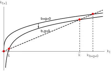
When $b=g=0$ we are back to the initial case without government. The Cobb-Douglas and log-utility specifications are characterised by two steady states:

• $\bar{k} > 0$, which is stable,
• $\bar{k}=0$, which is unstable.

With $b,g>0$ the $k_{t+1}$ curve moves downwards and the economy displays two steady states:

• $\bar{k}$, which is unstable,
• $\overline{k}$, which is stable.

There are two additional possibilities: in the first one, the $k_{t+1}$ curve is tangent to the 45 degree line. In that (unlikely) case, a unique steady state arises, but it is non-hyperbolic and we cannot infer its stability from the linearised version. Note: we know that the steady state is non-hyperbolic because $k_{t+1}$ evaluated at the steady state is tangent to a 45 degree line.

In the second case, if $b$ or $g$ are big enough, the economy has no steady state.