Steady state
We assume that the intertemporal equilibrium exists and is unique. As noted when characterising the uniqueness of the temporary equilibrium, assuming that $\sigma>1$ is a sufficient condition. Therefore, the dynamics of capital are given by:
$$k_{t+1} = \frac{1}{1+n}s(\omega(k_{t}), f^{\prime}(k_{t+1})).$$
Hence, $k_{t+1}$ is an implicit function of $k_{t}$:
$$k_{t+1} = g(k_{t}).$$
Steady states
The steady states of this economy can be found solving the previous equation for $k_{t+1} = k_{t}=\bar{k}.$
$$\bar{k} = \frac{1}{1+n}s\left(\omega(\bar{k}), f^{\prime}(\bar{k})\right).$$
Steady state with $\bar{k}=0$
A steady state with $\bar{k}=0$ is only possible if $f(0)=0$ or, equivalently, $\omega(0)=0.$ We may call this steady state an autarky steady state. In that case, since $\omega(0)=0$ and we know that individuals save a fraction of their income:
$$s(\omega(0), R(0)) < \omega(0) = 0.$$
Hence, given zero capital, savings are equally zero and capital remains there, constituting a steady state.
Alternatively, if it is possible to produce without capital (CES production function with large enough substitutability), the autarkic steady state does not exist.
Example of the autarkic steady state
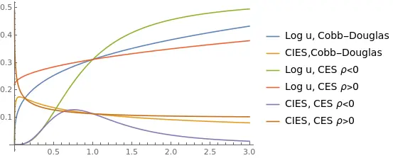
Take $F(K,L)=(\alpha K^{\rho} + (1-\alpha)L^{\rho})^{\frac{1}{\rho}}$ and $u( c ) = \log( c ).$ Furthermore, assume a low elasticity of substitution, $\rho « 0.$ In intensive form, production equals:
$$f(k_{t}) = (\alpha k_{t}^{\rho} + (1-\alpha))^{\frac{1}{\rho}}.$$ Wages and savings are:
$$\omega(k_{t}) = (1-\alpha)(\alpha k^\rho + (1-\alpha))^{\frac{1}{\rho}-1}$$ $$s_{t} = \frac{\beta}{1+\beta}w_{t}.$$
Then, capital accumulation becomes:
$$k_{t+1} = \frac{1}{1+n}\frac{\beta}{1+\beta}(1-\alpha)\left[\alpha k_{t}^\rho + 1 - \alpha \right]^\frac{1-\rho}{\rho}.$$
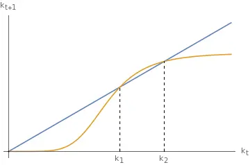
With low substitutability, $\rho < 0$, zero is always a possible steady state. There can be two additional, positive steady states depending on the curvature of $k_{t+1}.$
Similarly, the Cobb-Douglas case $\rho \rightarrow 0$ also has zero as a steady state. However, it is unstable.
Other steady state
The economy can also present interior steady states with $\bar{k}>0.$ Unlike the Ramsey model, here we can have stable and unstable steady states, as we shall see. Moreover, the configuration varies depending on the production and utility functions.
Stability of the steady state
This model can feature one or several steady states. This depends on the characteristics of the production and utility functions.
First, the dynamics of $k$ are monotonic: either continuously increase or decrease. This follows from assuming a unique intertemporal equilibrium, see also. This extra assumption also implies that the intermporal elasticity of substitution is not too small. In particular, we operationalise (p. 25 in de la Croix and Michel.) it as:
$$\forall c>0, \quad u^\prime( c ) + c u^{\prime \prime}( c ) \geq 0 \Leftrightarrow \sigma( c ) \geq 1.$$
Due to the fact the monotonicity of the dynamics, capital can converge either to $0,, \bar{k}\in (0,+\infty),, $ or $+\infty.$
The economy never goes to $k = +\infty$
This is equivalent to saying that starting with a a high level of capital $k_{0}$, the dynamics imply $k_{t+1} < k_{t}.$
First, we have that:
$$g(k) = \frac{1}{1+n}s(\omega(k),f^\prime(\underbrace{g(k)}_{k_{t+1}}))<\frac{\omega(k)}{1+n}.$$ This holds because savings $s$ are always a fraction of wages $\omega.$
Second, we show that:
$$\lim_{k \rightarrow +\infty}\frac{g(k)}{k} = 0.$$
To see the intuition for this limit, assume for a moment it holds. Then, it must be that for large enough $k,, g(k) = k_{t+1} < k_{t}$ and the dynamics are decreasing and converge to some $\bar{k}.$ In this case, $\bar{k}$ is the largest steady state, and because the dynamics are monotonic, the economy never goes to the other side of the steady state.
We show next that $\lim_{k \rightarrow +\infty}\frac{g(k)}{k} = 0.$ We do so by showing that $\lim_{k \rightarrow +\infty} \color{green}{\frac{\omega(k)}{k}} = 0.$
Detailed explanation
We start by noting that:$$\color{green}{\frac{\omega(k)}{k}} = \color{red}{\frac{f(k)}{k}} - \color{blue}{f^\prime (k)} \leftarrow \omega(k) = f(k) - f^\prime (k) k.$$
When $k \rightarrow +\infty$, the first term $\color{red}{\frac{f(k)}{k}}$ admits a positive limit, let’s call it $\mathcal{l}_{1}.$ This is because:
- $\color{red}{\frac{f(k)}{k}} > 0.$
- $\color{red}{\frac{f(k)}{k}}$ is decreasing: $$\frac{\partial \color{red}{\frac{f(k)}{k}}}{\partial k} = \frac{f^\prime(k)k-f(k)}{k^{2}} = - \frac{f(k) - f^\prime (k) k}{k^{2}} = - \frac{\omega(k)}{k^{2}} < 0.$$
The second term $\color{blue}{f^\prime (k)}$ is decreasing and positive, thus it admits a limit $\mathcal{l}_{2}$ when $k \rightarrow +\infty.$
Apply the mean value theorem evaluated at $k$ and $2k$:1
$$f(2k) - f(k) = (2k-k)f^\prime(k(1+\theta)), \quad \mathrm{with}, \theta \in (0,1).$$ Then, $$\frac{2f(2k)}{2k} - \frac{f(k)}{k} = f^\prime(k(1+\theta))$$ Taking the limit when $k \rightarrow +\infty$ we obtain $2\mathcal{l}_{1}-\mathcal{l}_{1} = \mathcal{l}_{2} \implies \mathcal{l}_{1} = \mathcal{l}_{2}.$
Finally,
$$\lim_{k \rightarrow + \infty}\color{green}{\frac{\omega(k)}{k}} =\lim_{k \rightarrow +\infty}\color{red}{\frac{f(k)}{k}} - \color{blue}{f^\prime (k)}= \mathcal{l}_{1} - \mathcal{l}_{2} = 0.$$
Since $\lim_{k \rightarrow +\infty} \color{green}{\frac{\omega(k)}{k}}=0$ and $\frac{g(k)}{k} < \color{green}{\frac{\omega(k)}{k}}$ then $\lim_{k \rightarrow +\infty}\frac{g(k)}{k} = 0.$ In conclusion, if the inital value of capital is large enough, the dynamics are decreasing and $k$ converges to an interior steady state $\bar{k}.$
Examples
Example 1: Log-utility and Cobb-Douglas
Suppose that $u(c,d) = \log ( c ) + \beta \log(d)$ and $f(k_t) = Ak_t^\alpha.$
The wage rate is given by $$w_t = f(k_{t}) - f^\prime (k_{t}) = (1-\alpha)Ak_{t}^\alpha$$
and the savings function is obtained solving $$u^\prime(w_{t} - s_{t}) = \beta R_{t+1} u^\prime (R_{t+1}s_{t}).$$
Rearranging and isolating $s$ we are left with the savings function
$$s_{t} = \frac{\beta}{1+\beta}w_{t}.$$
The dynamics are given by the capital accumulation law
$$k_{t+1} = \frac{1}{1+n}s_{t} = \frac{1}{1+n}\frac{\beta}{1+\beta}w_{t} = \frac{1}{1+n}\frac{\beta}{1+\beta}(1-\alpha)Ak_{t}^\alpha.$$
The model with log-utility and Cobb-Douglas production functions has two steady states: zero and a unique positive steady state. We can solve for them:
$$\bar{k} = \frac{1}{1+n}\frac{\beta}{1+\beta}(1-\alpha)A\bar{k}^\alpha \implies \bar{k} = \begin{cases} 0 \\\ \left(\frac{1}{1+n}\frac{\beta}{1+\beta}(1-\alpha)A\right)^{\frac{1}{1-\alpha}} \equiv \phi^\frac{1}{1-\alpha}\end{cases}.$$
Local dynamics: stability
We check the stability of the two steady states using the first derivative evaluated at the steady state. Note: in general we would use the Jacobian matrix, but the OLG model has only one equation in one variable.
Remember that, for a discrete-time system, a non-hyperbolic steady state is stable if it the determinant of the Jacobian (here the absolute value of the derivative) evaluated at the steady state is in the unit circle $(-1, 1).$
In our case:
$$g(k) = k_{t+1} = \frac{1}{1+n}\frac{\beta}{1+\beta}(1-\alpha)Ak_{t}^\alpha$$ $$g^\prime(k) = \frac{1}{1+n}\frac{\beta}{1+\beta}(1-\alpha)\alpha Ak_{t}^{\alpha-1}> 0.$$
Then
$$\bar{k}=0 \implies g^\prime (0) = + \infty \quad \rightarrow \mathrm{unstable}$$ $$\bar{k}=\phi^\frac{1}{1-\alpha} \implies g^\prime(\phi^\frac{1}{1-\alpha}) = \phi \alpha \phi^\frac{\alpha-1}{1-\alpha} = \alpha \in (0,1) \quad \rightarrow \mathrm{stable}.$$
Global dynamics
Suppose we have $k_{t+1} \geq k_{t}$. We show that the dynamics are bounded above by the steady state $\bar{k} = \phi^\frac{1}{1-\alpha}.$
$$k_{t+1} \geq k_{t} \Leftrightarrow g(k_t) \geq k_t \Leftrightarrow \phi k_t^\alpha \geq k_t \Leftrightarrow \phi \geq k_t^{1-\alpha} \Leftrightarrow \bar{k} \geq k_t.$$
Log-utility and CES technology
Under a CES specification, $y_{t} = A \left[ \alpha k_{t}^\rho + (1-\alpha) \right]^\frac{1}{\rho}, \rho \leq 1$ wages are given by $$\omega_{t} = (1-\alpha)\left[\alpha k^\rho + 1 -\alpha \right]^{\frac{1-\rho}{\rho}}.$$ Hence, the dynamics of capital are governed by:
$$k_{t+1} = g(k_t) = \frac{1}{1+n}s_{t} = \frac{1}{1+n}\frac{\beta}{1+\beta}A(1-\alpha)\left[\alpha k_{t}^\rho + 1 - \alpha\right]^\frac{1-\rho}{\rho}.$$ The curve $g(k)$ is increasing:
$$g^\prime (k) = \frac{\beta A (1-\alpha)}{(1+n)(1+\beta )}(1-\rho)\left[ \alpha k^\rho + 1 - \alpha \right]^\frac{1-2 \rho}{\rho}k^{\rho -1} > 0.$$
Depending on the value of $\rho$ we can have different configurations regarding the steady states. Ultimately, what matters is the concavity of the function $g(k_{t}).$
$$g^{\prime \prime}(k_t) = -\frac{1}{1+n}\frac{\beta}{1+\beta}A(1-\rho)\alpha\left[\alpha k^\rho+1-\alpha\right]^\frac{1-3\rho}{\rho}k^{\rho-2}\left(\rho \alpha k^\rho +(1-\alpha)(1-\rho)\right).$$
Unique steady state, $\bar{k} > 0$
If $\rho \in (0,1)$, the second derivative is clearly negative, and $g$ is concave. Moreover, $g(0)>0$, so $\bar{k} = 0$ cannot be a steady state:
$$g(k_{t}) = \frac{\beta A(1-\alpha)}{(1+n)(1+\beta)}(\alpha k^\rho + 1 - \alpha)^\frac{1-\rho}{\rho} \implies g(0)=\frac{\beta A(1-\alpha)^\frac{1}{\rho}}{(1+n)(1+\beta)}> 0.$$ In that case, the economy displays a unique steady state, and it is globally stable.
Unique $\bar{k}=0$ or multiple steady states
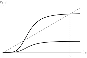
If $\rho < 0,$ the function $g(k)$ changes concavity. In particular, there exists a level $\hat{k}$ such that: $$g^{\prime \prime}(k) > 0, \mathrm{if} , k < \hat{k}.$$ $$g^{\prime \prime}(k) < 0, \mathrm{if} , k > \hat{k}.$$ with $$\hat{k} = \left( - \frac{(1-\alpha)(1-\rho)}{\rho \alpha}\right)^\frac{1}{\rho} > 0 , \mathrm{since}, \rho <0.$$ Moreover, $g(0)=0$ so $\bar{k}=0$ can be a steady state.
In this case, there are two sub-cases:
-
If $k_{t+1} < k_{t} \implies \frac{\omega(k)}{k} < (1+n)\frac{1+\beta}{\beta}$ then the trajectory of $k_{t+1}$ is always below $k$. Then, there is one unique steady state: $\bar{k}=0.$ The economy converges towards this unique steady state. We can derive the condition above from: $\begin{align} k_{t+1} < k_{t} & \implies \frac{1}{1+n}s\left(\omega(k_{t}),R_{t+1}\right) < k_{t} \implies \\\ \frac{1}{1+n}\frac{\beta}{1+\beta}w_t < k_{t} & \implies \frac{w_{t}}{k_{t}} < (1+n)\frac{1+\beta}{\beta}. \end{align}$
-
If there is some $k_{t+1} > k_{t} \implies \frac{\omega(k)}{k} > (1+n)\frac{1+\beta}{\beta}$ then there are two positive steady states $\bar{k}_{a} < \bar{k}_{b}$ plus the zero steady state $\bar{k}=0.$
- All trajectories starting at $k_0 < \bar{k}_{a}$ converge to $\bar{k}=0$ and $\bar{k}=0$ is locally stable in the range $[0,\bar{k}_{a}].$ The steady state with $\bar{k}=0$ is a poverty trap: whenever the economy starts with a low enough level of capital, it will always converge towards the $\bar{k}=0$ steady state.
- Trajectories starting at $k_0=\bar{k}_{a}$ remain at $\bar{k}_{a}$. This steady state is unstable.
- Finally, trajectories starting with $k_0 > \bar{k}_{a}$ converge towards $\bar{k}_{b}$, which is a locally stable steady state in $(\bar{k}_{a}, +\infty).$
Solved example
Suppose that production can be parametrized using the following Cobb-Douglas specification: \begin{equation} Y = F\left(K_t, L_t\right) = K_t^\frac{1}{2}L_t^\frac{1}{2}. \end{equation}
Furthermore, assume the following utility function: \begin{equation} u(c_t) = \frac{c_t^{1-\frac{1}{3}}-1}{1-\frac{1}{3}} \end{equation} where the intertemporal elasticity of substitution is $-3.$
We can compute production function, the wage and the interest in intensive form as: \begin{align} f(k_t) &= k_t^\alpha \\\ w_t &= f(k_t) - f^\prime(k_t) k_t = (1-\alpha) k_t^\alpha \\\ r_t &= f^\prime(k_t) = \alpha k_t^\frac{-1}{2} \end{align}
Similarly, the savings function can be derived from the Euler equation as follows: \begin{align} u^\prime(w_t - s_t) &= \beta R_{t+1} u^\prime(s_t R_{t+1}) \implies \\\ \implies (w_t -s_t)^\frac{-1}{3} &= \beta R_{t+1} (R_{t+1} s_t)^\frac{-1}{3} \implies \\\ \implies (w_t - s_t) &= \beta^{-3} R_{t+1}^{-2} s_t \implies \\\ s_t &= \frac{w_t}{1+\beta^{-3}R_{t+1}^{-2}} \end{align}
Therefore, the capital accumulation equation is: \begin{align} k_{t+1} &= \frac{1}{1+n} \frac{w_t}{1+\beta^{-3} R_{t+1}^{-2}} = \frac{1}{1+n} \frac{\frac{1}{2} k_t^\frac{1}{2}}{1+\beta{-3}\left(\frac{1}{2}k_{t+1}^\frac{-1}{2}\right)^{-2}} \implies \\\ k_{t+1} &= \frac{1}{1+n} \frac{\frac{1}{2} k_t^\frac{1}{2}}{1+4\beta^{-3} k_{t+1}} \implies \\\ \frac{1}{2} k_t^\frac{1}{2} &= (1+n)k_{t+1}\left(1+4 \beta^{-3} k_{t+1}\right) \implies \\\ k_{t+1} &= \frac{-(1+n) + \sqrt{(1+n)^2+8(1+n)\beta^{-3}k_t^\frac{1}{2}}}{8(1+n)\beta^{-3}} \end{align}
We can then show that the autarky steady state exists. Indeed, because we have $f(0) = 0$, then $\bar{k} = 0$ is a steady state. The economy has a second steady state, but solving for it explicitly is challenging becuase it involves a third degree polynomial. Nevertheless, let’s sketch the process, knowing that a steady state solves $k_t = k_{t+1} = \bar{k}.$ To simplify the notation, in what follows I will write $k$ instead of $\bar{k}.$ \begin{align} k = \frac{-(1+n) + \sqrt{(1+n)^2+8(1+n)\beta^{-3}k^\frac{1}{2}}}{8(1+n)\beta^{-3}} &\implies \\\ 1 + 8(1+n)\beta^{-3}k = \sqrt{1+8^{-3}k^\frac{1}{2}} &\implies \\\ 16 \beta^{-3}k + 64 \beta^{-6} k^2 = 8 \beta^{-3} k^\frac{1}{2} &\implies \\ k^\frac{1}{2}\left(8 \beta^{-3}k^\frac{3}{2} + k^\frac{1}{2} - 1\right) &=0 \end{align}
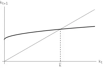
From here, it is obvious that $k = 0$ is a steady state, as we already knew. In principle, the part in brackes may have up to three solutions, but as said, these are hard to get. Instead, we can show that one and only one (real) solution can exist by studying the stability of the steady states. Moreover, the functional form we have is similar to a square root: we have the square root of something to the power $\frac{1}{2}$, so this means that the function will behave similar to $x^\frac{1}{4}.$ Thus, we can expect only a second steady state to exist.
The derivative of the dynamic function with respect to $k_t$ is:
\begin{equation} \frac{\partial k_{t+1}}{\partial k_t} = \frac{1}{4\sqrt{k_t}\sqrt{(1+n)\left(1+n+\frac{8\sqrt{k_t}}{\beta^{3}}\right)}} \end{equation}
When $k_t = k_{t+1} = 0$, the value of the derivative is $+\infty$, and thus, that steady state is non-stable. Moreover, for any value $k>0$, the derivative is between $0$ and $1$. Therefore, any other possible steady state is stable. Because the economy cannot converge to $k\rightarrow \infty$, and because all the potential steady states with positive capital are stable, this implies that only can exist. Otherwise, all of the would attract the dynamics, but this is impossible in this model: we must converge somewhere. In fact, the plot of the dynamics is as follows:
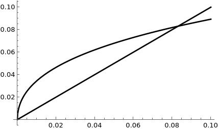
-
The mean value theorem states that, for a continuous function on $[a,b],$ there is a point $c \in (a,b)$ such that the derivative a $c, f^\prime( c)$ coincides with the slope of the secant between $a$ and $b, \frac{f(b) - f(a)}{b-a}.$ More information. ↩︎