Multiple intertemporal equilibria
In the OLG model, a unique intertemporal equilibrium arises if, for a given $k_t$, the equation
$$H(k_{t+1}) = k_{t+1} - \frac{1}{1+n}s\left(\omega(k_t), f^\prime(k_{t+1})\right) = 0$$
has a unique solution. We know that $\lim_{k \rightarrow 0}H(k) < 0$ and $\lim_{k \rightarrow +\infty}H(k) > 0,$ which guarantees the existence of at least one solution.
Hence, if the function $H$ is monotonously increasing, the solution is unique. This condition depends on the sign of:
$$\frac{\partial H(k_{t+1})}{\partial k_{t+1}} = 1 + \frac{1}{1+n}s^{\prime}_{R}f^{\prime \prime}(k_{t+1}).$$
We have different cases (check the notes on the savings function):
-
$s^\prime_{R} = 0$, which happens under log-utility. In this case, $s^\prime_{R} = 0 > \frac{1+n}{R^\prime(k_{t+1})}$ and $H(k_{t+1})$ is always increasing.
-
$s^\prime_{R} >0$, the intertemporal elasticity of substitution is greater than 1 and individuals are willing to trade off higher future consumption against present consumption. Savings increase to consume more in the future. Then, clearly $s^\prime_{R} > 0 > \frac{1+n}{R^\prime(k_{t+1})}.$
-
$s^\prime_{R} < 0$, we can have a non-monotonous capital path as $k_{t+1}$ can be increasing or decreasing with $k_{t}$.
Under case 3, the condition is not satisfied, multiple levels of $k_{t+1}$ solve the intertemporal equilibrium.
Non-monotonous dynamics
Note: Based on the lecture notes of Groth, pp. 92–93
Under case 3, the function $g(k)$ is backwards bending for some values of $k.$ This feature implies that there is more than one intemporal equilibrium, check also. We ruled out such a possibility assuming that $\sigma( c ) \geq 1$, this is, we imposed a large enough intertemporal elasticity of substitution.
If this is not the case and $s^\prime_{R}(\omega(k_t), R(k_{t+1})) < \frac{1+n}{R^\prime(k_{t+1})}$ then there are multiple temporary equilibriums.
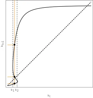
For instance, take an isoelastic utility function $u( c ) = \frac{c^{1-\frac{1}{\sigma}}-1}{1-\frac{1}{\sigma}}$ and a CES production with $A=20, , \alpha = \frac{1}{2}, , \beta = 0.3, , n = 1.097, , \sigma = 0.1, , \rho = -2.$ First, since $\sigma < 1$, it allows for the possibility of having multiple temporary equilibria. Second, we can verify that this is the case. For example, if $k_{t} = 1$, then:
$k_{t+1} = \frac{1}{1+n} s(\omega(k_{t}), R(k_{t+1})) \implies k_{t+1} = \begin{cases} 0.26 \\\ 1.234 \\\ 5.832 \end{cases}.$
In fact, for the entire range $k_{t} \in [0.76, 1.37]$ there is multiplicity of equilibria. Consequently, in all these cases we also have that $\frac{\mathrm{d}k_{t+1}}{\mathrm{d}k_t} < 0.$